A Bridgman Furnace Front Tracking Model

A

B

RIDGMAN

F

URNACE

F

RONT

T

RACKING

M

ODEL

U

D

,

T

C

S

E

,

M

M

D

A thesis submitted to the University of Dublin in partial fulfilment of the

requirements for the degree of Ph.D

by

Robin Patrick Mooney,

BE,

ME

Abstract

A Bridgman Furnace Front Tracking Model

Thesis by

Robin Patrick Mooney

Project Supervisor

Dr. Shaun McFadden

i

Declaration

I declare that this thesis has not been submitted as an exercise for a degree at this or any other University and it is entirely my own work.

I agree to deposit this thesis in the University’s open access institutional repository or allow the Library to do so on my behalf, subject to Irish Copyright Legislation and Trinity College Library conditions of use and acknowledgement.

ii

Summary

The ‘Bridgman’ furnace is widely used in industry and research to directionally solidify pure materials and alloys. The Bridgman process (for alloys) involves movement of the material through a tubular furnace consisting of hot and cold zones that are separated by a baffle or adiabatic gap. The hot zone is held at some temperature above the alloy liquidus, and the cold zone at some temperature below the alloy solidus, so that the material solidifies in a controlled manner in the space between. The sample is typically pulled through the furnace at a fixed rate to give steady solidification in a fixed temperature gradient (traditional ‘Bridgman’ mode); in this case, pulling rate changes can invoke transient solidification. In the Bridgman furnace ‘power down’ mode, the sample is stationary and the temperature of hot and cold zones is decreased at a fixed cooling rate. Steady solidification is achieved where both zone temperatures are decreased at the same cooling rate; transient solidification is achieved by applying different cooling rates in each zone.

The overall objective of this thesis has been to gain a better understanding of the solidification conditions, in particular, growth rate and temperature gradient, leading to Columnar to Equiaxed Transition (CET) in directionally solidified castings of gamma titanium alloys (TiAl) using a Bridgman furnace apparatus through mathematical modelling. Currently, TiAl alloys have the potential to replace nickel superalloys in the aerospace and automotive industries on account of their comparatively low density (≈50%) and equivalent strength and stiffness properties at high temperatures. Applications for TiAl alloys include: aero-engine turbine blades, turbocharger rotors and high performance engine valves. CET is an unwanted phenomenon that can occur in castings that adversely affects mechanical properties of cast components. Knowledge of the conditions that lead to CET in castings is therefore imperative. Experimental data for a TiAl multicomponent hypoperitectic alloy, directionally solidified in a Bridgman furnace procedure that involved transient Bridgman and transient power down modes of solidification (in series), was provided to the author of this thesis (by others) for the purposes of numerical modelling. Given this data, the overall thesis objective was broken down into five more manageable sub-objectives.

iii

The second objective was to verify the numerical model with an analytical model from the literature. Verification was achieved for the case of steady Bridgman solidification of a pure material (in this case pure titanium). Verification for transient Bridgman solidification of an alloy was not possible due to a lack of analytical models in the literature. The simulation results showed that the numerical model was first order accurate in space.

The third objective was to characterise a real Bridgman furnace apparatus in terms of heat transfer coefficients. The model was implemented in series with a discrete Proportional Integral Derivative (PID) controller to solve an inverse heat transfer problem using experimental data from static Bridgman furnace experiments performed with a hypoperitectic TiAl alloy. The model was adapted, in terms of latent heat release, for hypoperitectic growth. Simulation results showed that the furnace heat transfer coefficient at the sample circumference varied with axial position. The method applied is useful to other experimentalists, and to industry, since it avoids the difficult task of calculating heat transfer coefficients in the traditional manner where uncertainty exists in estimating the thermal emissivity values for the surfaces exchanging radiated heat. Further simulations were performed using the results without the PID controller to corroborate the method.

The fourth objective was to model unique experiments carried out in the same furnace where the transient ‘Bridgman’ and transient ‘power down’ modes were used in series to directionally solidify the same alloy at four different cooling rates. The model was used to simulate these experiments; one of which displayed CET in the sample microstructure; the others displayed ‘axial’ columnar to ‘radial’ columnar transition microstructures. Radial growth is an unwanted occurrence in CET experiments that tends to choke the undercooled region preventing the possibility of CET.

The fifth objective was to explain these microstructural observations using the model. The solidification conditions at the location of CET were estimated, namely; temperature gradient, growth rate, undercooling and undercooled region width. Comparisons were made with the other results. The simulation results highlight an important consideration for CET experiment designers; conditions that favour CET, e.g., low temperature gradient, also support radial columnar growth which can eliminate the possibility of CET. Reversal of radial heat flow at the sample circumference is proposed as a precursor for radial columnar growth.

iv

Acknowledgements

I would like to sincerely thank my supervisor, Assistant Professor Shaun McFadden, for his helpful guidance and support throughout this work. Shaun is an excellent supervisor. I would also like to thank Dr. Marek Rebow of Dublin Institute of Technology, and Dr. David Browne of University College Dublin, for offering their expert knowledge and opinion upon request.

I would like to thank the European Space Agency and Enterprise Ireland for funding this research under the PRODEX programme. Thank you to all my GRADECET research group partners for their cooperation. Particular thanks go to; Ulrike Hecht of ACCESS e.V. (RWTH Aachen University) for kindly welcoming me into the research group, and to Professor Juraj Lapin of the Institute of Materials and Machine Mechanics (Slovak Academy of Sciences) for offering their experimental data.

Thank you to my family, specifically to my parents, Maggi and Paraic, for their much appreciated assistance and encouragement. Finally—and most importantly—I would like to thank my wife, Victoria, for her continuous support and attention since the beginning of this work.

v

Preface

The work described in this thesis has been carried out by the author under the supervision of Dr Shaun McFadden in the School of Engineering at Trinity College Dublin. This work has been completed with financial assistance from the European Space Agency PRODEX programme, as part of the project: GRADECET (GRAvity DEpendence of Columnar to Equiaxed Transition in TiAl alloys). This work began on the 1st October 2010. The research described herein is original. The work of others has been drawn upon in places throughout the thesis, where this is so, acknowledgement is given to those other authors by way of reference. Some of the original material contained herein has already been published (or is submitted for publication). A list of these articles is given in the ‘Published Work’ section.

vi

Table of Contents

Declaration ... i

Summary ... ii

Acknowledgements ... iv

Preface... v

Table of Contents ... vi

List of Figures ... x

List of Tables ... xiii

Nomenclature ... xiv

Published Work ... xviii

1

Introduction

1

1.1

The Bridgman Furnace ... 1

1.1.1 Origin, history, and operation ... 1

1.1.2 Applications in industry ... 3

1.1.3 Applications in research ... 3

Experiments with transparent materials ... 3

Experiments with aerogel crucibles ... 4

Experiments with x-ray videomicroscopy ... 5

Analytical modelling ... 5

Numerical modelling ... 6

1.2

Thesis Objectives... 7

1.3

Thesis Structure ... 8

2

Literature Review

9

2.1

Solidification Morphologies ... 9

2.2

Dendritic Growth ... 10

2.2.1 Columnar growth ... 11

Analytical modelling ... 12

2.2.2 Equiaxed growth ... 14

Analytical modelling ... 14

2.2.3 Columnar to equiaxed transition (CET)... 15

Theories for the origin of equiaxed growth... 16

CET models ... 17

2.3

Eutectic Solidification (hypoeutectic path) ... 18

2.4

Peritectic Solidification (hypoperitectic path) ... 20

2.4.1 The peritectic reaction ... 20

2.4.2 The peritectic transformation ... 21

2.4.3 Growth models of peritectic solidification ... 21

2.5

Gamma Titanium Aluminide Alloys ... 21

2.5.1 The TiAl binary alloy phase diagram ... 23

2.5.2 Current studies involving multicomponent gamma TiAl alloys ... 24

2.5.3 Effect of further alloying elements (Nb, B, C) ... 25

2.5.4 Applications of gamma titanium alloys ... 26

Aerospace applications ... 26

vii

Processing Routes ... 27

2.6

The Front Tracking Model (FTM) ... 27

2.6.1 The heat equation ... 27

2.6.2 Nucleation ... 28

2.6.3 Tracking the front ... 28

2.6.4 Dendrite kinetics ... 30

2.6.5 Latent heat ... 30

2.6.6 Eutectic solidification in the FTM... 32

2.6.7 Thermophysical properties ... 33

2.7

Front Tracking Methods with Convection ... 33

2.8

Conclusion to the Literature Review ... 35

2.9

Scope of the Current Research ... 36

3

Model Development

37

3.1

The Biot Number ... 37

3.2

Bridgman Furnace Front Tracking Model (BFFTM) ... 37

3.2.1 The heat equation ... 38

3.2.2 The domain ... 39

3.2.3 The heat fluxes ... 40

3.2.4 Movement of the front ... 41

Bidirectional requirement ... 41

Status flags ... 42

3.2.5 Nucleation, thermophysical properties, and numerical stability ... 44

3.2.6 Code structure ... 44

3.3

Modelling Bridgman Solidification of Al–7wt.%Si ... 46

3.3.1 A transient solidification problem ... 46

3.3.2 Properties of Al–7wt.%Si ... 46

3.3.3 Simulation details ... 47

3.4

Modelling Results ... 48

3.4.1 Grid convergence study ... 48

3.4.2 Simulation 1: Results ... 48

3.4.3 Simulation 2: Results ... 49

3.5

Discussion ... 51

3.6

Conclusion ... 51

4

Order Verification

52

4.1

Definition of ‘Verification’ ... 52

4.2

Order Verification Method ... 52

4.2.1 Theoretical order of accuracy ... 53

4.2.2 Observed order of accuracy ... 53

4.2.3 Order verification procedure ... 54

4.3

Bridgman Solidification ... 56

4.3.1 The Bridgman procedure ... 56

4.3.2 The test problem ... 57

4.4

Modelling ... 57

4.4.1 Mathematical model ... 57

4.4.2 Analytical solution ... 58

4.4.3 Numerical solution ... 60

Implementation of the BFFTM... 60

viii

Growth law for high purity titanium ... 61

Fraction of solid ... 62

4.5

Results ... 62

4.6

Discussion... 64

4.7

Conclusion ... 66

5

Characterisation of a Bridgman Furnace

67

5.1

Bridgman Furnace Heat Transfer Coefficients ... 67

5.2

Methodology... 68

5.2.1 Experimental method ... 68

The experiment apparatus ... 68

The experimental procedure... 70

5.2.2 Mathematical model and the numerical implementation ... 70

Application of the mathematical model to the experiment apparatus ... 70

The heat transfer coefficients ... 72

Model domain ... 72

Boundary conditions ... 73

PID method for solving the inverse heat transfer problem ... 73

Determining the heat transfer coefficient at the crucible circumference75

5.3

Simulation Input Parameters ... 75

5.3.1 Geometrical properties... 75

5.3.2 Numerical parameters ... 76

5.3.3 Controller parameters ... 76

5.3.4 Material properties ... 76

Thermophysical properties ... 76

Dendrite kinetics ... 77

Solid fraction estimation ... 77

5.4

Results ... 78

5.4.1 Experimental results ... 79

5.4.2 Numerically processed results ... 79

Heat flux and heat transfer coefficients at the domain boundaries ... 79

Heat flux at the circumference of the sample... 79

Heat transfer coefficient at the circumference of the crucible ... 80

5.5

Discussion... 81

5.5.1 Discussion of results ... 81

Experimental results ... 81

Heat flux and heat transfer coefficients at the domain boundaries ... 81

Heat flux at the circumference of the sample... 82

Heat transfer coefficient at the circumference of the crucible ... 84

Average heat transfer coefficient at the circumference of the crucible . 85 5.5.2 Discussion of the 1-dimensional heat flow assumption ... 86

5.5.3 Discussion on convection in the liquid ... 86

5.5.4 Discussion on heat flow in the crucible ... 87

5.6

Conclusion ... 87

6

Power Down Experiment Modelling

89

6.1

Methodology... 89

6.1.1 Experiment apparatus ... 89

6.1.2 Experimental procedure ... 90

6.1.3 Sample analysis ... 92

ix

6.2

Results ... 94

6.2.1 Experimental results ... 94

6.2.2 Numerical results... 96

6.3

Discussion ... 98

6.3.1 Summary of experiment results ... 98

6.3.2 Radial columnar growth ... 99

6.3.3 Columnar to equiaxed transition ... 102

6.3.4 Convection in the melt ... 103

6.4

Conclusion ... 104

7

Discussion

105

7.1

Background Theory on Dendrite Kinetics for Alloy 455 ... 105

7.2

Sensitivity Analysis of Dendrite Kinetics ... 106

7.3

Discussion Summary ... 109

8

Conclusions and Future Work

110

8.1

Conclusions ... 110

8.2

Future Work ... 113

Bibliography

117

Appendix

130

A.1

Derivation of the 1-Dimensional Heat Flow Equation ... 130

A.2

Discretisation of the 1-Dimensional Heat Flow Equation ... 132

A.3

Taylor Series Formulations for First Order Derivatives ... 135

x

List of Figures

Fig. 1.1 Schematic of a typical Bridgman furnace and temperature profile. ... 2

Fig. 2.1 Solid–liquid interface morphologies in directional solidification: (a) planar, (b) cellular and (c) dendritic. ... 9

Fig. 2.2 Thermal fields for columnar (a) and equiaxed (b) dendrites in alloys, adapted from [3]. .. 11

Fig. 2.3 (a) Columnar dendritic growth into a superheated liquid with imposed temperature gradient and (b) equiaxed dendritic growth into an undercooled melt with temperature T∞. ... 12

Fig. 2.4 Columnar to equiaxed transition visible in a longitudinal section of a cylindrical sample (70 mm in diameter and 150 mm in length) of Al–7wt.%Si [47]. ... 15

Fig. 2.5 Typical binary eutectic alloy phase diagram and hypoeutectic dendrite morphology, adapted from [4]. ... 19

Fig. 2.6 A binary peritectic phase diagram and hypoperitectic dendrite morphology. The inserts illustrate a peritectic reaction (upper) a peritectic transformation (lower), adapted from [4]. ... 20

Fig. 2.7 Specific strength versus temperature for various alloys [73]. ... 22

Fig. 2.8 GEnx aircraft engine [77]. ... 23

Fig. 2.9 Titanium-aluminium phase diagram [84]... 24

Fig. 2.10 (a) Schematic of dendritic growth. (b) Front tracking model applied to dendritic growth. ... 29

Fig. 2.11 Evolution of nucleation sites showing early columnar growth and impingement [87]. .... 29

Fig. 2.12 Captured volume. ... 31

Fig. 3.1 Schematic of heat transfer occurring in a moving rod. ... 38

Fig. 3.2 Bridgman furnace front tracking model domain and co-ordinate system. ... 39

Fig. 3.3 (a) Disc shaped control volumes (b) control volume with heat flux shown. ... 40

Fig. 3.4 Typical progress of the columnar front marker with status flag values shown. ... 43

Fig. 3.5 Bridgman furnace front tracking model algorithm flowchart. ... 45

Fig. 3.6 Simulation 1: Evolution of a steady-state temperature profile. ... 49

Fig. 3.7 Simulation 1: Thermal history in the adiabatic zone and change in front position. ... 49

Fig. 3.8 Simulation 2: Evolution of temperature profile with two step changes in pulling rate. ... 50

Fig. 3.9 Simulation 2: Thermal history in the adiabatic zone and change in front position. ... 50

Fig. 4.1 Code verification procedure, adapted from Knupp and Salari [134]. ... 55

Fig. 4.2 Schematic of a Bridgman furnace. ... 56

Fig. 4.3 Evolution of temperature profile resulting from step change in pulling rate. ... 63

Fig. 4.4 Temperature profile for comparison of analytical and numerical solutions. ... 63

Fig. 5.1 Schematic of the Bridgman furnace apparatus. ... 69

Fig. 5.2 Schematic of the cold (a) and hot (b) regions of the Bridgman furnace apparatus. ... 71

xi

Fig. 5.4 Control system block diagram with negative feedback loop to control CV temperature. .. 73

Fig. 5.5 Ideal PID controller with derivative filter. ... 74

Fig. 5.6 Block diagram for the calculation of the heat transfer coefficient, h3. ... 75

Fig. 5.7 Solid fraction to temperature relationship for alloy 455 as estimated using Thermocalc® [165] via the ‘Modified Scheil Module’. ... 78

Fig. 5.8 Experiment temperature profiles at various heater settings. ... 79

Fig. 5.9 Heat flux at the sample circumference versus axial position. ... 80

Fig. 5.10 Heat transfer coefficient at the crucible circumference versus axial position. ... 80

Fig. 5.11 Measured temperature profile for experiment E.1 (top) and heat flux at the sample circumference calculated via the PID controller (bottom) to give the same simulated temperature profile. ... 83

Fig. 5.12 Experimental and simulated temperature profiles using the average heat transfer coefficient... 85

Fig. 6.1 Schematic of the Bridgman furnace apparatus. ... 90

Fig. 6.2 Schematic plot of the process signals: pulling rate, controlled cooling rate, and thermocouple temperature, all versus time for the experimental procedure. ... 91

Fig. 6.3 (a) The physical model and (b) the numerical model of the Bridgman furnace apparatus aligned with (c) a typical sample temperature profile result. ... 93

Fig. 6.4 Images of etched and polished samples with primary -phase microstructure regions identified as follows: U–unmelted, C–axial columnar, R–radial columnar, and E–equiaxed. ... 94

Fig. 6.5 Detailed images of samples I, III, and IV showing the typical microstructural regions observed. ... 95

Fig. 6.6 Dendrite tip growth rate versus front position. ... 97

Fig. 6.7 Dendrite tip undercooling versus front position. ... 97

Fig. 6.8 Dendrite tip growth rate versus tip temperature gradient. ... 98

Fig. 6.9 Undercooled region width versus front position. ... 98

Fig. 6.10 Axial and radial columnar growth in the sample cooled at 50 °C/min. ... 99

Fig. 6.11 Effect of radial heat flow direction on front shape: (a) desirable convex front shape, (b) unfavourable concave front shape. ... 100

Fig. 6.12 The width of the undercooled region ahead of a columnar dendrite. ... 102

Fig. 7.1 Columnar dendrite tip growth rate versus dendrite tip undercooling for values of growth coefficient and undercooling exponent in Table 7.1. ... 106

Fig. 7.2 Simulated front position (a), columnar tip growth rate (b) and tip temperature gradient (c) all versus time. ... 107

Fig. 7.3 Simulated tip growth rate (a) and tip temperature gradient (b) versus front position. ... 107

Fig. 7.4 Simulated columnar tip growth rate versus tip temperature gradient. ... 108

xii

Fig. A.1 Conservation of energy in a cylindrical elemental fixed volume. ... 130

Fig. A.2 Control volume ‘i’. ... 132

xiii

List of Tables

Table 3.1 Control volume status flags used to activate latent heat flux. ... 43

Table 3.2 Material properties for Al–7wt.%Si [56]. ... 47

Table 3.3 Grid convergence study results. ... 48

Table 4.1 Thermophysical properties for high purity titanium and other modelling input data. ... 57

Table 4.2 Order verification simulation results ... 64

Table 4.3 Effect of increasing the thermal range for phase change. ... 65

Table 5.1 Geometrical properties used in all simulations. ... 75

Table 5.2 Numerical parameters used in all simulations. ... 76

Table 5.3 Ideal PID controller settings for all simulations. ... 76

Table 5.4 Polynomial coefficients used to estimate thermophysical properties of the sample alloy and crucible, adapted from Egry [162] and Touloukian [163]. ... 77

Table 5.5 Experiment reference numbers with hot and cold region reference temperatures. ... 78

Table 5.6 Heat flux, heat transfer coefficients, and extrapolated temperature at the domain boundaries. ... 79

Table 6.1 Experimental results. ... 95

Table 6.2 Measured axial columnar transition positions and corresponding numerical results. ... 96

Table 6.3 Simulated positions of radial heat flow reversal. ... 101

xiv

Nomenclature

A cross sectional area [m2]

b dendrite growth rate undercooling exponent [–] Bi Biot Number [–]

c specific heat capacity at constant pressure [J/kg·°C] C dendrite growth rate coefficient [m/s·°Cb]

C0 original alloy composition [wt.%]

Ctip composition of the liquid at the tip [wt.%]

d captured volume of mush in a control volume [m3] D derivative controller signal [–]

Dsolute diffusivity of solute in the liquid [m

2 /s] e error [°C]

E latent heat generated per unit volume [W/m3] f heat flow [W]

F radiation view factor [–] gS volumetric solid fraction [–]

G temperature gradient [°C/m] GC concentration gradient [wt.%/m]

h heat transfer coefficient [W/m2·°C] H enthalpy [J]

I integral controller signal [–] Iex equiaxed index [m

2 ·°C]

k thermal conductivity [W/m·°C] kpart partition coefficient [–]

Kc controller gain [–]

l

LA adiabatic zone length, or baffle thickness [m]

Lchar characteristic length [m]

LM latent heat of fusion per unit mass [J/kg]

Lmol molar latent heat of fusion [J/mol]

LV latent heat of fusion per unit volume [J/m

3 ] ml alloy liquidus slope [°C/wt.%]

n order of numerical error [–] N low pass filter variable [–] NCVs number of control volumes [–]

NE numerical error [°C] p perimeter [m]

po observed order of accuracy [–]

xv Pe, PeT thermal Péclet number [–]

PeC solutal Péclet number [–]

q heat flux [kW/m2] Q heat flow [W] r radius [m]

R dendrite tip radius [m]



t time [s]

T temperature [°C] u pulling rate [m/s] Ub bulk undercooling [°C]

v growth rate [m/s] V volume [m3]

V growth velocity of peritectic -phase [m/s] x axial position, or Cartesian abscissa [m]

x’ axial position with respect to the columnar dendrite tip [m] X dimensionless axial position [–]

y Cartesian ordinate [m]

 thermal diffusivity [m2/s]

 solid–liquid interface energy [J/m2]

 Gibbs–Thomson coefficient [m·K]

l elemental volume thickness [m]

Sf m

molar entropy of fusion [J/mol·K]

t numerical time step [s]

T bath undercooling [°C]

TC solutal undercooling [°C] TK kinetic undercooling [°C] TR curvature undercooling [°C] TT thermal undercooling [°C] Ttip dendrite tip undercooling [°C] x control volume thickness [m]

y control volume height [m]

 crystalline anisotropy strength [–]

 refinement ratio [–]

K attachment kinetics coefficient [m/s·°C]

ξC function of solutal Péclet number [–]

 density [kg/m3]

 Stefan–Boltzmann constant, 5.6703732 × 10−8 [W/m2·K4]

xvi

D derivative time constant [s]

I integral time constant [s]

ΩC solutal supersaturation [–] ΩT thermal supersaturation [–]

 thermal range [°C]

Sub-scripts

1 at the sample axis, or baffle boundary (when used as subscript to x)

2 at the sample crucible boundary, or baffle boundary (when used as subscript to x) 3 at the exposed crucible wall

4 at a reference position

5 at the heater (or crystalliser) surface a advancement

adv advection c conduction (net) cru crucible

C cold zone CV control volume

e east face

euc eutectic exp experimental H hot zone i spatial label

j element label in a multicomponent alloy l liquidus

L liquid

m melting

nuc nucleation per peritectic rad radial s solidus S solid sim simulated t thickening tip dendrite tip

w west face

x axial direction ∞ infinity (far away)

xvii m temporal label

xviii

Published Work

Journal Articles

R. P. Mooney, U. Hecht, Z. Gabalcová, J. Lapin, and S. McFadden, “Directional solidification of a

TiAl alloy using a combined Bridgman & power down technique,” 2014. (Submitted.)

R. P. Mooney and S. McFadden, “Order verification of a Bridgman furnace front tracking model in steady state,” Simulation Modelling Practice and Theory, vol. 48, pp. 24–34, 2014.

R. P. Mooney, S. McFadden, Z. Gabalcová, and J. Lapin, “An experimental–numerical

method for estimating heat transfer in a Bridgman furnace,” Applied Thermal Engineering, vol. 67, no. 1–2, pp. 61–71, 2014.

R. P. Mooney, S. McFadden, M. Rebow, and D. J. Browne, “A Front Tracking Model for

Transient Solidification of Al–7wt%Si in a Bridgman Furnace,” Transactions of the Indian Institute of Metals, vol. 65, no. 6, pp. 527–530, 2012.

Conference Proceedings

R. P. Mooney and S. McFadden, “Sensitivity analysis of dendritic growth kinetics in a Bridgman furnace front tracking model,” in 4th International Conference on Advances in

Solidification Processes, 2014.

R. P. Mooney and S. McFadden, “The Role of Verification in Computer Modelling: A Case Study in Solidification Processing,” in 31st International Manufacturing Conference, 2014, pp. 173–180.

J. Lapin, Z. Gabalcová, U. Hecht, R. P. Mooney, and S. McFadden, “Columnar to Equiaxed

Transition in Peritectic TiAl Based Alloy Studied by a Power-Down Technique,” Materials Science Forum, vol. 790–791, pp. 193–198, 2014.

R. P. Mooney and S. McFadden, “An investigation into Bridgman furnace solidification,” in 30th International Manufacturing Conference, 2013, pp. 375–383.

R. P. Mooney, S. McFadden, M. Rebow, and D. J. Browne, “A front tracking model of the

MAXUS-8 microgravity solidification experiment on a Ti-45.5at.% Al-8at.%Nb alloy,” IOP Conference Series: Materials Science and Engineering, vol. 27, no. 1, p. 12020, 2012.

1

Chapter 1

1 Introduction

Introduction

In this chapter the Bridgman furnace is introduced, its operation explained in detail, and examples of its applications in industry and in research are given. Particular focus is given to examples of the Bridgman furnace in research. The thesis aims and objectives are outlined. This is followed by a description of the thesis chapter structure in the context of the aims and objectives given.

1.1

The Bridgman Furnace

1.1.1

Origin, history, and operation

The ‘Bridgman Furnace’ takes its name from the 1946 Nobel Prize winning Physicist; Percy W. Bridgman. In the 1920’s, Bridgman developed a technique of lowering a cylindrical crucible at a fixed rate along the axis of a vertical tubular furnace, held at a fixed temperature, to produce single crystal materials [1]. The technique was later modified by Donald C. Stockbarger, in the 1930’s, to produce large single crystals of lithium fluoride [2], where a high temperature gradient was required for successful growth. To achieve higher gradients, a second tubular heat sink is employed, separated from the furnace heater by a thin annular baffle. The resulting solidification procedure is known as the Bridgman-Stockbarger technique, Bridgman solidification, or the Bridgman method. Many variations of the original set-up have since been developed, however, the principle of operation has remained the same.

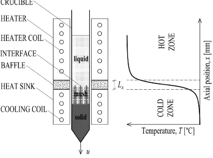
Figure 1.1 shows a schematic of a typical Bridgman furnace with the characteristic temperature profile in the sample material. The arrangement allows for solidification to occur primarily in one direction (in this case, in the direction of the sample axis), and in a positive temperature gradient, i.e., dT/dx>0. Any such procedure can be referred to as directional solidification. The material, contained in a crucible or ampoule, is lowered through the furnace from the hot zone into the cold zone at some pulling rate, u. The heater is maintained at a temperature, TH, above the equilibrium liquidus temperature for the material, Tl; and the heat sink is

held at a temperature, TC, below the material equilibrium solidus temperature, Ts. The heater and

heat sink are separated by a baffle of thickness, LA, thereby establishing a temperature gradient in

the material, ~ (TH−TC)/LA. The key advantage of the method is that solidification can be performed

2

Fig. 1.1 Schematic of a typical Bridgman furnace and temperature profile.

When very large temperature gradients are required, the heat sink is sometimes achieved by surrounding the crucible in a liquid metal bath or via water cooling methods. The size of the temperature gradient in the sample is adjusted by changing the baffle thickness, LA, or by varying

the heater temperature, TH, and heat sink temperature, TC, appropriately.

Where it is desirable to grow a single crystal, the crucible usually has a sharp pointed bottom. In pure materials, normally a planar (flat) solid–liquid interface forms. With alloys, however, the solidification interface can take on a planar, cellular (curved) or dendritic (treelike) shape; the latter of which is most common [3]. In dendritic solidification the material forms a ‘mushy’ zone (a combination of solid and liquid). The directional solidification occurring in the figure is typical for that of an alloy, i.e., the fully solid part of the sample is separated from the fully liquid part by a mushy region made up of dendritic solid and interdendritic liquid [4]. The interface in the figure is given by the mush–liquid boundary. During steady growth, the interface forms somewhere between the hot and cold zones and moves at the same rate (but in the opposing direction) as the pulling rate.

3

at the interface; in other words, the cooling rate applied by the heater must equal the cooling rate applied by the heat sink for steady growth to occur.

1.1.2

Applications in industry

The Bridgman method can be used to produce single crystal materials; via careful crucible design or alternatively, by placement of a seed crystal at the crucible tip [5]. By ‘single crystal’ (or mono-crystal) it is meant that the entire material sample is made up from one continuous crystal lattice throughout; there are no grain boundaries. Careful control of the cooling process, possible using the Bridgman method, can ensure that the crystal lattices align and solidify. Such materials benefit from exceptional properties that are desirable for use in industry. The most common application is in the semiconductor industry where single crystal silicon is used in the production of microprocessors and wiring where extremely low electrical and thermal resistance is desirable. Silicon mono-crystals are widely used in the photovoltaics industry where the material is used to maximise energy conversion efficiency in solar panels [6]. Single crystal lithium fluoride is used in the optics industry (for UV transmission windows) and also in X-ray detectors, on account of its transparency to shortwave ultra-violet radiation [7]. It is possible to cast some alloys (nickel-based superalloys, or titanium alloys) using the Bridgman method as single crystals, for example, in the manufacture high pressure turbine blades. The resultant casting offers superior resistance to creep needed to endure the harsh centrifugal forces of the application at high temperature [8].

Bridgman solidification can be effective in metal purification [9]. This is because most impurities are more soluble in the liquid phase than in the solid phase, therefore, the solidification front pushes the impurities out into the liquid melt during growth. The solidification procedure is carried out a number of times, each time the top section of the sample (containing all the impurities) is cut off before repeating the procedure.

1.1.3

Applications in research

Experiments with transparent materials

In 1965 Jackson and Hunt first published details about experiments on transparent compounds as analogues for freezing metals [10]. Using the Bridgman method they observe that the existence of transparent materials provide an opportunity to make direct observations of the phenomena that determine the structure of cast metals. For example, it was previously impossible to examine criteria for dendrite growth kinetics by direct observation.

4

larger values of dendrite tip undercooling leading to thinner arm necks; a condition favourable for dendrite detachment.

The relationship of growth rate and primary dendrite arm spacing was investigated by Ding et al. [12] using ethanol and acetone transparent alloys of succinonitrile. The effect of step increments in growth rate (with a fixed temperature gradient), and changes in temperature gradient (at a fixed growth rate) are examined in this study. It is determined that primary dendrite arm spacing is heavily dependent on growth rate and temperature gradient, and that the historical values for these parameters have a major influence on the resulting arm spacing. In other words, the transient effects of varying the pulling rate or temperature gradient are notable.

A combined experimental–numerical study was performed by Simpson et al. [13] where convection in the melt is considered for growth of pure succinonitrile in a Bridgman furnace. Digital cameras are employed to observe planar growth and flow paths due to convection using suspended particles in the melt. The solid–liquid interface shape and velocity are measured which compares well with two and three dimensional numerical models.

Transparent material experiments using the Bridgman method have more recently been carried out in microgravity environments where convection effects in the melt are absent. Bergeon et al. [14] and Weiss et al. [15] give detailed accounts of a Bridgman solidification experiment using succinonitrile alloys carried out on the International Space Station (ISS) where three dimensional spatio–temporal evolution of solidification is observed. The aim of this experiment was to provide unique benchmark data for validation of numerical phase field models, and also to describe the physics of interface pattern selection, and to determine the criteria that govern planar to cellular, and cellular to dendritic transitions.

Recently, studies by Mogeritsch and Ludwig [16][17][18] describe in-situ observations of a peritectic transparent organic material during solidification in an experimental micro-Bridgman furnace. Interphase spacing of the  and  peritectic phases is measured as a function of growth velocity for a fixed composition, and as a function of composition for a fixed growth velocity.

Experiments with aerogel crucibles

5

Experiments with x-ray videomicroscopy

Mathiesen and Arnberg [22] have taken a major step further into the observation of the solidification process using the Bridgman method. Experiments were carried out at the European Synchotron Radiation Facility (ESRF) where samples of Al–30wt.%Cu were directionally solidified whilst undergoing high resolution fast acquisition x-ray imaging. Using this method, it was possible to examine the microstructure evolution and local liquid constitution during solidification through a 2-dimensional field of view (1.35  1.35 mm2) at intervals of 0.45 s. The images were further analysed to extract information about interface morphology, dendrite tip growth rate at the solid–liquid interface and constitutional undercooling at the dendrite tip. Whilst steady dendrite growth is not realised in these experiments, they highlight the advantages of using x-ray radiography in understanding solidification phenomena, as well as providing important modelling data for dendritic growth models.

Using the same technique, a subsequent study [23] focuses on observations of dendritic fragmentation resulting from local solute enrichment during the directional solidification of Al– 20wt.%Cu. It is found that the accumulation of solute at the root of tertiary dendrite arms can lead to a decrease in melting temperature of the solid–liquid interface, consequently resulting in remelting of the arm leading to detachment, i.e., fragmentation. This phenomenon is important in understating the problem of columnar to equiaxed transition (CET) in castings.

More recently, further work [24] has been done using x-ray radiography to investigate coarsening in the mushy zone in Bridgman solidification of Al–30wt.%Cu. In this study, secondary dendrite arm spacing (SDAS) is measured during acceleration and deceleration of the solidification front. The observations show that the proximity of primary dendrites does not affect SDAS during deceleration of the solidification front. On the contrary, during accelerations of the solidification front secondary dendrite arms coarsened more, and were more likely to produce tertiary dendrite arms.

A study by Reinhart et al. [25] was carried out where unrefined Al–3.5wt.%Ni and boron refined Al–5wt.%Ti–1wt.%B alloys were solidified in a vertical Bridgman furnace. In situ real-time imaging of the solidification behaviour of thin samples (40 mm in length, 6 mm in width, and 150 m to 200 m in thickness) of both materials is obtained by synchrotron x-ray radiography at the ESRF. A sharp jump in pulling rate is applied in order to provoke a CET in the sample. Several key observations in relation to the CET are made, for example; the evolution of undercooling ahead of the columnar tip, and the CET blocking mechanism. Importantly, this study outlines a method to calculate the evolution of nuclei density between successive images for equiaxed growth, a task only possible through x-ray radiography.

Analytical modelling

6

material properties are assumed constant in the liquid and the solid phases. Convection in the melt is assumed negligible. The model assumes a planar growth interface only. Latent heat is accounted for using a 1-dimesional analysis with the Stefan condition applied to solve for interface position. The heat transfer coefficients at both heaters are assumed equal.

Naumann [27] presents a similar model suitable for use with small sample diameters (less than 10 mm) with the addition of an adiabatic zone and separate thermophysical properties for solid and liquid. Naumann further extends this work as a hybrid analytical–numerical 2-dimensional model [28] valid for long thin samples and very low pulling velocities (~100 mm/h) which are suitable for single crystal growth. The effect of adiabatic zone length and curvature of isotherms is analysed.

Gandin, Schaefer and Rappaz [29] present an analytical model for predicting the growth of a single dendritic grain envelope solidifying in a Bridgman furnace where a fixed thermal gradient and isotherm velocity is assumed. The model is applied in two dimensions. The Kurz Giovanola and Trivedi [30] (KGT) model for dendritic growth is applied giving a quadratic relation of undercooling for growth rate. The model is limited because the growth kinetics are valid for low levels of undercooling, latent heat is assumed negligible, and the model cannot not cope with interactions of the single grain envelope with the mould wall or with another grain.

Numerical modelling

Brown and Kim [31] apply a fully implicit axisymmetric numerical model, to solve for heat transfer, melt convection and species transport in a vertical three zone Bridgman furnace. The purpose of the study is to accurately model crystal growth with a view to reducing radial segregation in the crystals. The model results are compared to experimental data for a dilute Ga–Ge alloy. The stagnant film model [32] and Scheil model [33] for solute transport at the solid–liquid interface are used in this analysis. It is found that the intensity of mixing in the melt has a strong bearing on the level of radial segregation observed.

An experimental study by Neugebauer and Wilcox [34] shows that a booster heater located between the hot zone and the adiabatic zone of a Bridgman furnace can be used to thermally stabilise (or destabilise) the effect of convection depending on the power applied to the booster. It is found that convection effects in vertical Bridgman solidification could be avoided by applying low pulling rates, using dilute alloys, or by operating in a microgravity environment.

7

assumptions include: equal heat capacity and density in the liquid and solid, fixed but separate thermal conductivity in the solid and liquid, fixed heat transfer coefficients at the hot and cold heaters, and large length-to-diameter ratio of the sample.

Su, Jemian and Overfelt [36] carried out an experimental study where sudden changes in pulling rate are investigated in Bridgman solidification of Al–Cu alloys. The model of Fu and Wilcox [35] is tested alongside a similar model by Saito and Hirata [37]. It is reported that the latter model is in better agreement with the experiments carried out.

Eiken et al. [38] have carried out a case study of phase field simulations of Bridgman solidification of a Ti–Al–Nb alloy to examine microstructure morphology in early peritectic growth. The effect of varying critical undercooling for growth and adding grain refiners is simulated and compared to experimental data for three different values of aluminium content. The study is considered qualitative given the lack of reliable data for diffusion coefficients in the melt and interfacial energies.

Li et al. [39][40] have carried out a two-part study where a fixed grid front tracking model was applied to Bridgman growth of succinonitrile. The model assumes a planar solidification front. The model considers buoyancy induced convection, applied moving boundary conditions to simulate the heater movement, and assumed fixed but separate thermophysical properties for the solid and liquid phases.

1.2

Thesis Objectives

The work presented in this thesis has been motivated by a need to understand the pertinent solidification conditions that may, or may not, produce a columnar to equiaxed transition in gamma titanium aluminide castings. The author is currently a member of a research group, GRADECET (described later in Section 2.5.2), that shares this motivation. One specific task, imparted by this research group to the author, emerged as follows:

‘To numerically model terrestrial Bridgman furnace experiments for directional solidification in a

gamma titanium aluminide alloy where the Bridgman method is combined in series with the power

down technique; and to provide enlightenment into the experimental results obtained using the

model’.

The above task is the overall objective of this thesis; however, it is appropriate to break this task down into several, more manageable, objectives as follows:

1. To develop a numerical model for transient Bridgman furnace solidification that incorporates a front tracking model from the literature.

8

3. Characterise the Bridgman furnace experimental apparatus (in terms of heat transfer coefficients) using the numerical model and experimental data.

4. Apply the numerical model to the directional solidification experiments (carried out in the same furnace) where the Bridgman method is combined in series with a power down method.

5. Use the numerical model to explain microstructural observations in the experiment samples and to provide insight into the experiment process.

1.3

Thesis Structure

9

Chapter 2

2 Literature Review

Literature Review

In this chapter a review of relevant literature is provided. Firstly, a summary of solidification morphologies commonly occurring in metallic systems is given (in Section 2.1). This is followed by a review of dendritic growth in metallic alloys (in Section 2.2). Eutectic and peritectic alloy solidification is explained (in Section 2.3 and Section 2.4, respectively). Peritectic gamma titanium aluminide alloys are then reviewed (in Section 2.5). This is followed by a detailed look at a front tracking model for dendritic solidification from the literature (in Section 2.6), and a short review of front tracking methods that account for convection (in Section 2.7). The chapter is concluded (in Section 2.8) and the scope of the current work, as part of this thesis, is given (in Section 2.9).

2.1

Solidification Morphologies

The morphology (shape) of the solid–liquid interface during solidification of metallic or non-metallic systems can be categorised into one of three commonly occurring types: planar, cellular, and dendritic, as shown in Fig. 2.1. In each case shown, growth occurs in the positive x-direction and the material temperature, T, is shown by a thick black line. The liquid regions (white areas labelled ‘L’) have a higher temperature than the solid regions (grey areas labelled ‘S’). In other words, growth is occurring in a positive temperature gradient (dT/dx>0). This is known as directional solidification [3]. In metallic systems, the shape of the interface is primarily determined by the diffusion of heat and mass.

10

For pure metallic materials, the diffusion of heat controls the interface shape. Pure materials solidify with a planar interface when directionally solidified. A perturbation, i.e., a disturbance in shape, on the planar surface in Fig. 2.1(a) will find itself in liquid hotter than the melting point of the pure material. The perturbation will therefore melt back; in this case, latent heat generated is extracted via the solid. Pure materials can take on a dendritic morphology (not shown here), for example, in the case of a thermal dendrite growing in an undercooled melt, where solidification occurs in a negative temperature gradient and latent heat is extracted via the liquid. Surface perturbations, in this case, find themselves in liquid at a lower temperature than the local solidus temperature of the alloy and therefore can grow (eventually into a dendritic shape).

In alloys, however, the interface morphology is mainly controlled by the diffusion of mass— specifically the diffusion of solute—such that all three interface types in Fig. 2.1 can occur. Tiller et al. [41] were the first to elucidate the link between the diffusion of solute and stability of a planar interface. In their analysis they determine the constitutional supercooling criterion to predict the stability of a planar interface in the directional solidification of binary alloys (having a partition coefficient kpart < 1), as follows:

,

C l

G

m

G



where G is the temperature gradient in the liquid, ml is the slope of the liquidus line from the

equilibrium phase diagram for the alloy, and GC is the concentration (solute) gradient in the liquid.

If G>mlGC then a planar interface will remain stable, Fig. 2.1(a). If G<mlGC then a planar interface

is unstable and any perturbation on the planar surface will grow into a dendritic form, Fig. 2.1(c). In this case, the liquid near the interface is constitutionally supercooled. (Note that in the literature ‘supercooled’ is often replaced by ‘undercooled’ and ‘constitutional undercooling’ is equivalent to ‘solutal undercooling’.) Finally, if G≈mlGC, then a cellular interface may form, Fig. 2.1(b), which

rapidly leads to dendritic form if G is decreased. Dendritic growth is the most common of the three interface morphologies for metallic alloy systems.

2.2

Dendritic Growth

Dendritic (from the Greek word dendron, meaning tree) growth refers to the formation and subsequent growth of treelike primary crystals during the solidification of a material where the solidifying shape is branched like a tree, with primary, secondary and tertiary dendrite arms [42]. The solid–liquid interface for most metallic alloy systems is atomically rough. The structure of the liquid phase is similar to that of the solid phase; so atoms in the liquid encounter an abundance of potential bonding sites. This leads to apparent random attachment of atoms during solidification giving a rough and uneven interface at the atomic scale, in other words, non-faceted growth. This occurs when Sf

m

< 2



11

solid–liquid interface energy, . The most successful interface shape in this case is dendritic. Two dendritic growth scenarios possible in metallic alloys systems are considered next: dendritic columnar growth and dendritic equiaxed growth. This is followed by a section dealing with the occurrence of both of these scenarios in a single casting, i.e., columnar to equiaxed transition.

2.2.1

Columnar growth

In a given casting, columnar dendrites begin growth at or near the mould wall, nucleating heterogeneously at the mould itself or emanating from chill grains. They grow with a preferred crystallographic direction—opposite to the direction of heat flow—into the liquid melt with a dendritic growth morphology. The latent heat generated (by solidification) is extracted via the solid columnar dendrite, to the mould wall. This can only occur when the temperature gradient at the solid–liquid interface, i.e., at the dendrite tip, is positive, as shown in Fig. 2.2(a). This means that the temperature of the liquid ahead of the columnar dendrite tip is higher than the temperature of the tip itself. Note the direction of the columnar growth rate, vtip, is opposite to the direction of heat

flow, Q. The equilibrium liquidus temperature, Tl, is plotted as a function of position, x. At the

dendrite tip Tl is reduced, primarily due to local enrichment of the liquid by solute rejected at the

tip (solutal undercooling), and secondly due to the capillarity effects given by the curvature of the solid–liquid interface (curvature undercooling). The total difference between the equilibrium liquidus temperature for the alloy and the temperature at the tip is known as the dendrite tip undercooling, Ttip. This is the usually the primary driving force for growth in metallic alloys. At

temperatures below the equilibrium solidus temperature, Ts, the columnar dendrite is fully solid.

Columnar growth is also known as constrained growth, since the growth of the dendrites is constrained or fixed by the rate of heat extraction.

12

Fig. 2.3 (a) Columnar dendritic growth into a superheated liquid with imposed temperature gradient and (b) equiaxed dendritic growth into an undercooled melt with temperature T∞.

Analytical modelling

Analytical models of columnar growth focus on steady-state solutions to the solutal diffusion equation from the point of view of an observer fixed at the dendrite tip. Consider the moving coordinate system, with the origin fixed at the dendrite tip, as shown in Fig. 2.3(a), where x’ is the position within the moving reference frame. The thermal gradient at the dendrite tip, G, is imposed by the process. The cooling conditions (rate of heat extraction) constrain the growth rate of the dendrite, however, the temperature at which growth occurs is primarily a function of solute rejection and hence alloy composition. Solute is rejected at the tip during growth leading to a snowplough effect of solute so that a concentration gradient exists in the liquid ahead of the tip. This leads to a local decrease of equilibrium liquidus temperature of the liquid at the tip, increasing back to its original value for the alloy of Tl(C0) at some distance away, as shown in Fig. 2.3(a),

where the dashed line shows Tl as a function of x’[9].

The curvature of the tip itself also creates a departure from equilibrium leading to step decrease of the local equilibrium liquidus temperature at the tip. Columnar growth is often considered a solute-diffusion-controlled process given that curvature effect is less significant at low solidification velocities [42], however, both are considered here. The dendrite tip undercooling,

Ttip, is made up by solutal undercooling, TC, and curvature undercooling, TR, such that;

.

R C

tip

T

T

T











Considering solutal diffusion only, Ivantsov [43] found a solution to the steady-state diffusion equation for the growth of a dendrite tip having a paraboloid of revolution shape. Critically, this choice of shape is self-preserving during growth. The solution equates the dimensionless solutal supersaturation, ΩC, to a function of the solutal Péclet number, Iv(PeC),

known as the Ivantsov function, as follows:

,

)

(

C



Iv

Pe

13

where PeC=vtipR/2Dsolute is the solutal Péclet number (ratio of solutal advection rate to solutal

diffusion rate), R is the dendrite tip radius and Dsolute is the diffusivity of solute in the liquid, and

where ΩC=(Ctip−C0)/(Ctip(1−kpart)), Ctip is the composition of the liquid at the tip, C0 is the original

binary alloy composition and kpart is the alloy partition coefficient (assumed less than unity), and

finally the Ivantsov function is defined as,

,

)

(

)

exp(

)

(

Pe

Pe

Pe

E

Pe

Iv



where E1(PeC) is the exponential integral function. Equation (2.3) can be rewritten in terms of

solutal undercooling, TC, by rearranging for Ctip and assuming straight lines for liquidus and

solidus on the alloy phase diagram to give,

.

)

(

)

1

(

1

)

(

)

(

Pe

Iv

k

Pe

Iv

T

T

k

T











This analysis provides a set of Péclet numbers for a given level of solutal undercooling and, as a result, only pairs of values for growth rate and dendrite tip radius are determined.

The curvature undercooling is given by TR=2/R where  is the Gibbs–Thomson

coefficient (the ratio of the solid–liquid interface energy to the entropy of fusion). By substituting this expression and equation (2.5) into equation (2.2) yields the dendrite tip undercooling for columnar growth from the analytical model of Kurz et al. [30]. In this model—known as the KGT model—the authors use the marginal stability criterion of Langer and Müller-Krumbhaar [44], where it is assumed that dendrites grow at the critical wavelength of stability for a planar interface. The marginal stability criterion introduces a stability parameter (a constant) * such that; 1/*∝vtipR

2

, in this case *=1/(22, thus providing a second relationship for growth rate and radius, and thereby permitting the calculation of explicit values of growth rate for any given dendrite tip undercooling. Under the KGT model, the solution to the following quadratic transcendental equation gives the columnar dendrite tip growth rate,





0

,

)

(

)

1

(

1

)

1

(

2































G

Pe

Iv

k

D

k

C

m

v

D

Pe

v





where ml is the slope of the liquidus line from the phase diagram, ξC is a function of solutal Péclet

number (that approaches unity at low Péclet numbers or π2/kpartPeC at high Péclet numbers), and G

is the mean temperature gradient at the interface.

14

2.2.2

Equiaxed growth

Equiaxed growth in metallic alloys occurs from within an undercooled melt. That is, the melt has a temperature lower than the equilibrium liquidus temperature for the alloy. Once nucleation has occurred, an equiaxed dendrite (for cubic metallic systems) grows equally along all six crystallographic axes of the primary phase, hence the term equi-axed. Referring to Fig. 2.2(b), the growth direction in this case is the same as the direction of heat flow. Latent heat generated on solidification is transported away from the solid–liquid interface into the undercooled liquid and subsequently to the mould wall through the liquid. The temperature gradient at the dendrite tip must be negative for equiaxed growth. In a similar manner to the case of columnar growth, the liquidus temperature at the dendrite tip is reduced due to solute enrichment and because of capillarity effects. However, since the thermal gradient at the tip is negative, an additional contribution (thermal undercooling) is included in the overall bath undercooling, T. Note that the equiaxed dendrite is isothermal during growth; however the thermal gradient in the liquid is not known a priori. Equiaxed growth is also referred to as free growth or unconstrainedgrowth since the growth rate is limited only by the available undercooling, as opposed to the rate of heat extraction [42].

Analytical modelling

In equiaxed growth, modelling solutal diffusion, capillarity effects and thermal diffusion must be considered, since the latent heat generated is transported away from the dendrite tips via the liquid. Consider a moving coordinate system, fixed the tip of a growing equiaxed dendrite, as shown in Fig. 2.3(b). The undercooled melt provides an additional driving force for growth, i.e., thermal undercooling TT, not seen in columnar growth, such that the total bath undercooling is given by,

.

R C

T

T

T

T

T















The solution to the thermal diffusion problem is analogous to that of solutal diffusion where the thermal Péclet number, PeT, and thermal supersaturation, ΩT, replace the their solutal counterparts

in the Ivantsov solution as follows:

,

)

(



Iv

Pe



where PeT=vtipR/2 is the thermal Péclet number,  is the thermal diffusivity (ratio of thermal

conductivity to volumetric heat capacity), ΩT=(Ttip−T∞)/(LV/cL), T∞ is the far field bath temperature, LV is the latent heat of fusion per unit volume, and cL is the specific heat capacity of the liquid. The

thermal undercooling, TT, can then be calculated as,

.

)

(

L V

T

Iv

Pe

c

L

T





15

and capillarity effects—already discussed for columnar growth—to get the following expression for total bath undercooling:

.

2

)

(

)

1

(

1

1

1

)

(

R

Pe

Iv

k

C

m

Pe

Iv

c

L

T

V

































This equation fails to yield distinct values for growth rate and dendrite tip radius; rather, only pairs of their product are available by its solution. The LGK model applies the marginal stability criterion to give the following expression for dendrite tip radius,

,

)

(

)

1

(

1

)

1

(

*

/

Pe

Iv

k

k

C

m

Pe

c

L

Pe

R















where * is introduced as the stability criterion parameter, equal to 1/42 (when using the marginal stability criterion). For a given value of bath undercooling, equation (2.10) and equation (2.11) can be solved using a numerical iteration method to determine explicit values for the growth rate and dendrite tip radius.

2.2.3

Columnar to equiaxed transition (CET)

In most castings either a columnar or equiaxed grain structure occurs. Sometimes, however, both columnar and equiaxed grain structures can be observed. This important phenomenon is known as columnar to equiaxed transition (CET). A CET is said to occur when the progress of constrained (columnar) grain growth is blocked by the nucleation and subsequent growth of unconstrained (equiaxed) grains [9]. Figure 2.4 shows an image of a CET in an aluminium–silicon alloy (Al–7wt.%Si), taken from a directional solidification study by Gandin [47]. The elongated columnar grains on the left hand side of the image are distinctive from the equiaxed grains on the right hand side. A detailed account of theory and models for CET is given by Spittle [48].

16

Fully columnar or fully equiaxed grain structure is normally desired in completed cast components so that consistent mechanical properties are achieved throughout the casting. For example, castings with a columnar grain structure are used in directionally solidified turbine blades in order to reduce creep at high temperatures. Whereas, fully equiaxed cast components are used in applications where strength is important, to improve feeding, or reduce the possibility of hot tearing. It is therefore vital to understand the conditions that produce a CET in order to avoid it as necessary.

Theories for the origin of equiaxed growth

Hutt and St John [49] reviewed several theories regarding the mechanism by which equiaxed grains form and lead to a CET in castings.

The Constitutional Supercooling hypothesis is proposed by Winegard and Chalmers [50]. During columnar growth, a region of constitutionally undercooled (or ‘supercooled’) liquid forms ahead of the dendrite tips, i.e., the region enclosed by the dashed line and the temperature profile line in Fig. 2.3(a), due to an accumulation of solute in the liquid. It is assumed that, once a critical level of undercooling is exceeded, heterogeneous nucleation of equiaxed crystals can occur on unknown particles in the undercooled melt. If the equiaxed grains are sufficient in size or number the progress of the columnar growth will be stopped.

The Big Bang hypothesis of Chalmers [51] proposes that very large numbers of equiaxed crystals can nucleate in the supercooled region at or near the mould walls of a casting during pouring, in a manner similar to chill grain formation. However, the equiaxed grains are transported throughout the melt as a result of convection due to pouring. Equiaxed grains that survive remelting can then continue to grow when they encounter constitutionally undercooled regions in the melt.

The Dendrite Arm Remelting theory is proposed by Jackson et al. [52] in a study observing solidification experiments of transparent alloy analogues. They noticed necking (thinning) of secondary dendrite arms due to solute build up. Latent heat release, convection, or fluctuations in growth rate could lead to fragmentation of these secondary arms which subsequently get transported by buoyancy forces into the melt where they grow as equiaxed grains.

The Showering of Dendrite Particles theory is proposed by Southin [53] in a study that observed the solidified macrostructure of Al–Cu laboratory ingots. This theory suggests that dendritic crystals form at the free surface of an ingot could somehow break away and sink into the melt where upon they meet other grains growing from the mould wall. In this study, the observed equiaxed grains were comet shaped since they tended to grow in line with the columnar grains on impingement.

17

in a similar manner to the Big Bang hypothesis, have narrow necks that can be broken by thermal convection forces before they fully solidify. The broken equiaxed dendrite would separate and be transported into the melt where they may continue to grow as free dendrites in undercooled regions. Hutt and St John conclude by stating that all of the above mechanisms can occur depending on alloy composition, casting conditions and the types of substrates available for nucleation of equiaxed grains in the melt. However, in the case of directional solidification of an alloy using the Bridgman method—with an imposed positive temperature gradient—and in the absence of convection effects or fluctuations in the cooling conditions, the origin of equiaxed grains is most likely to occur under the constitutional supercooling hypothesis.

CET models

A review