Dirichlet Compound Multinomials Statistical Models
Paola Cerchiello, Paolo Giudici
Department of Economics and Management, University of Pavia, Pavia, Italy Email: [email protected]
Received August 31, 2012; revised September 31, 2012; accepted October 6, 2012
ABSTRACT
This contribution deals with a generative approach for the analysis of textual data. Instead of creating heuristic rules for the representation of documents and word counts, we employ a distribution able to model words along texts considering different topics. In this regard, following Minka proposal (2003), we implement a Dirichlet Compound Multinomial (DCM) distribution, then we propose an extension called sbDCM that takes explicitly into account the different latent topics that compound the document. We follow two alternative approaches: on one hand the topics can be unknown, thus to be estimated on the basis of the data, on the other hand topics are determined in advance on the basis of a prede- fined ontological schema. The two possible approaches are assessed on the basis of real data.
Keywords: Textual Data Analysis; Mixture Models; Ontology Schema; Reputational Risk
1. Introduction
With the rapid growth of on-line information, text cate- gorization has become one of the key techniques for handling and organizing data in textual format. Text cate- gorization techniques are an essential part of text mining and are used to classify new documents and to find in- teresting information contained within several on-line web sites. Since building text classifiers by hand is diffi- cult, time-consuming and often not efficient, it is worthy to learn classifiers from experimental data. In this pro- posal we employ a generative approach for the analysis of textual data. In the last two decades many interesting and powerful contributions have been proposed. In parti- cular, when coping with the text classification task, a researcher has to face the well-known problem of poly- sems (multiple senses for a given words) and synonyms (same meaning for different words). One of the first effective model able to solve those issues is represented by Latent semantic analysis (LSA) [1]. The basic idea is to work at a semantical level by reducing the vector space through Singular Value Decomposition (SVD), producing not sparse occurrence tables that help in discovering associations between documents. In order to establish a solid theoretical statistical framework in this context, in [2] a probabilistic version of LSA (pLSA) has been proposed, also known as the aspect model, rooted in the family of latent class models and based on a mixture of conditionally independent multinomial distributions for the couple words-documents. The intention from the introduction of pLSA was to offer a formal statistical framework, helping the parameter interpretation issue as
well. By the way the goal was achieved only partially, in fact the multinomial mixtures, which components can be interpreted as topics, offer a probabilistic justification at words but not at documents level. In fact the latter are represented merely as list of mixing proportions derived from mixture components. Moreover, the multinomial distribution presents as many values as there are in the training documents and therefore it learns topic mixture on those trained documents. The extension to previously unseen documents is not appropriate since there can be new topics. In order to overcome the asymmetry between words and documents and to produce a real generative model, [3] proposed the LDA (Latent Dirichlet Allo- cation). The idea of such new approach emerges from the concept of exchangeability for the words in a document that unfolds in the “bag of words” assumption: the order of words in a text is not important. In fact the LDA model is able to capture either the words or documents ex- changeability unlike LSA and pLSA. On the other hand
LDA is a generative model in any sense since it posits a Dirichlet distribution over documents in the corpus, while each topic is drawn from a Multinomial distri- bution over words. However note that [4] in 2003 have shown that LDA and pLSA are equivalent if the latter is under a uniform Dirichlet prior distribution. Obviously
topics by replacing the Dirichlet random variable with the logistic normal distribution. Unlike LDA, CTM pre- sents a clear complication in terms of inference and parameter estimation since the logistic normal distri- bution and the Multinomial are not conjugate. To bypass the problem, the most recent alternative is represented by the Independent Factor Topic Models (IFTM) introduced in [6]. Such proposal makes use of latent variable model approach to detect hidden correlations among topics. The choice to explore the latent model world allows to choose among several alternatives ranging from the type of re- lation, linear or not linear, to the type of prior to be spe- cified for the latent source. For sake of completeness is important to mention another interesting research path focusing on the burstiness phenomenon, that is the ten- dency of rare words, mostly, to appear in burst. The above mentioned generative models are not able to cap- ture such peculiarity, that instead is very well modelled by the Dirichlet Compund Multinomial model (DCM). Such distribution was introduced by statisticians [7] and has been widely employed by other sectors like bioinfor- matics [8] and language engineering [9]. An important contribution in the context of text classification was brought by [10] and [11] that profitably used DCM as a bag-of-bags-of-words generative process. Similarly to
LDA, we have a Dirichlet random variable that generates a Multinomial random variable for each document from which words are drawn. By the way, DCM cannot be considered a topic model in a way, since each document derives specifically by one topic. That is the main reason why [12] proposed a natural extension of the classical topic model LDA by plugging into it the DCM distri- bution and obtaining the so called DCMLDA. Following this line of thinking, we move from DCM approach and we propose an extension of the DCM, called “semantic- based Dirichlet Compound Multinomial” (sbDCM), that permits to take latent topics into account. The paper is organized as follows: in Section 2 we show the Dirichlet Compound Multinomial (DCM) model, in Section we propose an extension of the DCM, called “semantic- based Dirichlet Compound Multinomial” (sbDCM), in Section 4 we show how to estimate the parameters of the different models. Then, in Section 5 we assess the pre- dictive performance of the two distributions by using seven different classifiers. Finally we show the different classification performance according to the knowledge on the topics T (known or unknown).
2. Background: The Dirichlet Compound
Multinomial
The DCM distribution is a hierarchical model: on one hand, the Dirichlet random variable is devoted to model the Multinomial word parameters ; on the other hand,
the Multinomial variable models the word count vectors
x comprising the document. The distribution function of the DCM mixture model is:
dp x p x p
. (1) where p x
is the Multinomial distribution:
\ 1
! W w. x w W
w w w
n p x
x
(2)in which x is the words count vector, xw is the count
for each word and w the probability of emitting a word i; therefore a document is modelled as a single set of
words (“bag-of-words”). The Dirichlet distribution
w
p is instead parameterized as:
1 1
\ 1
.
w
W w W w
w W
w w w
p
(3)with
w the Dirichlet parameter vector for words, as consequence the whole set of words (“bag-of-bags”) is modelled. Thus a text (a document in a set) is modelled as “bag-of-bags-of-words”. Developing the previous in- tegral we obtain:
1
\
1 1
!
W
w W
w w
W W
w w
w w w
w w
x n
p
x x
w
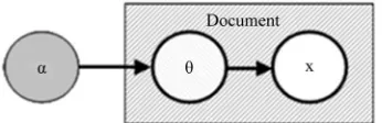
(4)In Figure 1 we reportthe graphical representation of
the DCM model. From another point of view, each Multinomial is linked to specific sub-topics and makes, for a specific document, the emission of some words more likely than others. Instead the Dirichlet represents a general topic that compounds the set of documents and thus the DCM could be also described as “bag-of-scaled- documents”. The added value of the DCM approach consists in the ability to handle the “burstiness” of a rare word without introducing heuristics [13]. In fact, if a rare word appears once along a text, it is much more likely to appear again.
When we consider the entire set of documents
D , where each document is independent and identified by its count vector,
D
x x1, , , xN
, the likelihood of the [image:2.595.338.511.660.716.2]whole documents set (D) is
1 1 1 1 1 N d d W w N W w w Wd w w
d w w
p D p x
x x
w (5)where xd is the sum of the counts of each word in the
document d-th (xdw) and xdw the count of word w-th for
the document d-th. Thus the log-likelihood is:
1 1 1
1 1
log
log log
log log
N W W
w w
d w w
N W
dw w w
d w p D x x w
(6)The parameters can be estimated by a fixed-point iteration scheme, as described in Section 4.
3. A Semantic-Based DCM
As explained in Section 2, we have a coefficient w for
each word compounding the vocabulary of the set of documents which is called “corpus”. The DCM model can be seen as a “bag-of-scaled-documents” where the Dirichlet takes into account a general topic and the Multinomial some specific sub-topics. Our aim in this contribution is to build a framework that allows us to insert specifically the topics (known or unknown) that compound the document, without losing the “burstiness” phenomenon and the classification performance. Thus we introduce a method to link the coefficients to the hypothetic topics, indicated with
i , by means of a function F
dim a
which must be positive in since the Dirichlet coefficients are positive. Note that usually and, therefore, our proposed approach is parsimonious. Substituting the new function into the integral in Equation (1), the new model is:
dim b
d ,p x
p x p F
(7)We have considered as function F() a linear combina- tion based on a matrix D and the vector . D contains
information about the way of splitting among topics the observed count vectors of the words contained in a diagonal matrix A and is a vector of coefficient
(weights) for the topics. More specifically we assume that: 1 11 1 1 , , , T
W W W
t
T
w d
A D
w d d
D A D
1 T d (8)
1 t T F D (9) Note that: T t
t
d
w t
with T the number of Topics; wt w wt;
dwtis the coefficient for word w-th used to define the
degree of belonging to topic t-th and by which a portion of the count of word w-th is assigned to that particular topic t-th.
d w d
By substituting this linear combination into Equation (4), we obtain the same distribution but with the above mentioned linear combination for each :
1 1 1 1 !W T T
wt t W w wt t
w t t
W W T T
w
w w wt t wt t
w w t t
p x
d x
n
x x d d
d
(10) This model is a modified version of the DCM, hence- forth semantic-based DCM (sbDCM), and the new log- likelihood for the set of documents becomes:
1 1 1
* 1 1
log
log log
log log
N W T W T
wt t w wt t
d w t w t
N W T T
dw wt t wt t
d w t t
p D
d x d
x d d
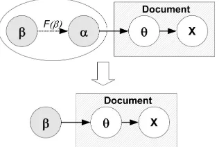
(11)In Figure 2 we report the graphical representation of
the new model where the ’s are substituted by a function of the ’s. An important aspect of the proposed approach is represented by the number T of topics to be inserted into the sbDCM that can be:
Figure 2. Hierarchical representation of sbDCM model.
A priori known (i.e. fixed by field experts).
The first case will be treated in Section 5.1, in parti- cular since it is not always possible to know in advance the number of latent topics present in a corpora, it be- comes very useful to build a statistical methodology for discovering efficiently and consistently a suitable num- ber of topics. In this case the number of topics T can be considered a random variable. Thus, we use a segmen- tation procedure to group the words in order to create groups of words sharing common characteristics that can be considered as latent topics. The analysis is completed by choosing the best number of groups and a distance matrix is used to set the membership percentage (dwt) of
each word to each latent topic. The second case will be treated in Section 5.2 and proposes to exploit the sbDCM
model by employing a priori knowledge based on on- tological schemas that describe the relations among con- cepts with regards to the general topics of the corpora. The ontology structure provides the set of relations among the concepts to which can be associated a certain number of key words, by a field expert(s). Thus, we want to use the classes of a given ontology and the associated key words to define in advance the number T of topics.
4. Parameters Estimation
There are several methods to maximize the log-like- lihood and to find the parameters associated with a DCM: simplified Newton iteration, the Expected Maximization method and the maximization of the simplified likelihood (called “leave-one-out” likelihood, LOO). Among them, the most general and flexible algorithm is the Expected Maximization (EM). The EM algorithm is an iterative procedure able to compute the maximum-likelihood es- timates whenever data are incomplete or they are consid- ered complete but not observable (latent variables) [14].
In general, considering p X Z
,
the joint prob- ability distribution (or probability mass function) whereX is the incomplete (but observable) data set and Z the missing (or latent) data, we can calculate the complete maximum likelihood estimation of model parameters by means of the EM algorithm. We obtain an overall
complexity reduction for what concerns the calculation of observed maximum-likelihood (ML) estimates. The goal is achieved by alternating the expectation (E-step) of the likelihood with the latent variables as if they are observed and the maximization (M-step) of the likelihood function found in the E-step. With the result of the
M-step we update the new parameters new that are used
again in the cycle, by starting from the E-step, until we reach a fixed degree of approximation of the observed likelihood which increases step by step moving towards the maximum (that could be local) [15]. The EM can be built in different ways. One possibility is to see the EM
as a lower bound maximization where we alternate the
E-step to calculate an approximation of the lower bound for the log-likelihood and maximize it in the M-step until a stationary point (zero gradient) is reached. If we are able to find a lower bound for the log-likelihood we can maximize it via a fixed-point iteration; in fact it is the same principle of considering the EM as a lower bound maximization. In our context, for the DCM, the lower bound with log
p D
is the following quantity:
1k
k k dw w w k k w
w w N W W
k k
d w w
d w w
x
x
(12)this allows us to use a fixed point iteration whose steps are:
1k
k k dw w w k k w
w w N W W
k k
d w w
d w w
x
x
(13)
where xd is the sum of the counts of each word in the
document d-th
xdw
, xdw the count of word w-th forthe document d-th and k w
the Dirichlet coefficient for word w at the k-th step. The algorithm is stopped when a degree of approximation is reached. The iteration starts with wequals to the occurrence percentage of the word
w-th in the corpus. The estimated parameters, as said before, have an important characteristic: they follow the “burstiness” phenomenon of words. In fact the smaller w is, the more “burstiness” effect is contained within a
word, as revealed in Section 5.
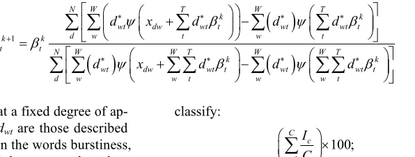
1
N W T W T
k k
wt dw wt t wt wt t
d w t w t
k k
t t N W W T W W T
k k
wt dw wt t wt wt t
d w w t w w t
d x d d d
d x d d d
(14)
As before we stop the iteration at a fixed degree of ap- proximation and the coefficients dwt are those described
in Section 3. The new ’s maintain the words burstiness, as we shall show in Section 5 and they are used to clas- sify the document by employing a Naive Bayes clas- sifier. For our applications, in the next section we have used for both models a value of of 10−10. The iteration
starts with t equals to the percentage of each single
cluster obtained by the grouping analysis of vocabulary words.
5. Model Performance
In this section we describe the evaluation of the different classifiers by using the parameters estimated from the
DCM distribution. Thus, our training data set is com- pound of 6436 documents with a vocabulary (already filtered and stemmed) of 15,655 words so we have to es- timate 15,655 parameters. The parameter is able to model the “burstiness” of a word. In fact, the smaller the parameters are, the more bursty the emission of words is. This phenomenon is characteristic of rare words, therefore coefficients are, on average, smaller for less counted words. The average value of the overall pa- rameters is 0.0342, the standard deviation is 0.1087 and the maximum and minimum values are respectively 6.6074 and 0.0025. Once the coefficient vector of ’s is obtained we employ seven different classifiers, three of which are described in [13] (normal (N), complement (C) and mixed (M). The remaining ones are proposed as the appropriate combination of the previous ones, in order to improve their characteristics. Those new classifiers are set in function of the number of words that a test-docu- ment has in common with the set of documents that compound a class; in this way we create a classifier in function of the number of words in common. Thus we analyze the following additional classifiers: COMPLE- MENT + MIXED + NORMAL (CMN), COMPLE- MENT + NORMAL (CN), COMPLEMENT + MIXED (CM), MIXED + NORMAL (MN).
In order to evaluate the classification performance we employ three performance indexes:
Ind1: The proportion of true positive over the total number of test-documents:
1
100;
D d d
TP D
Ind2: The proportion of classes that we are able to
classify:
1
100;
C c c
I C
where Ic is an indicator that we set 1 if at least one
document of the class is classified correctly, otherwise we set 0.
Ind3: The proportion of true positive within each class over the number of test documents present in the class:
1
1
100;
C c c c
TP C M
where Mc is the number of test-documents in each class,
TPc is the number of true positive in the class and C the
number of topics (46).
For the four combined classifiers such indexes have been calculated by varying the number of words in com- mon between the test document and the class. In particu- lar for our test we have used three different thresholds for the number of words (n): 15, 10 and 5. For example, we indicate with the initials CMn the classification rule that
employs classifier C when the number of common words are less or equal to n and classifier M when the number of words in common is more than n. Instead, the initial
CMNn.m identifies the using of classifier C until n, the
classifier N over m and the classifier M between n and m. For the data at hand the number of words in common between the two sets (training and evaluation set) varies between 1 and 268. The above mentioned combination is based on the following idea: if the number of words in common between the bag of words and the correct class is low, then the most information content is in the com- plement set. Otherwise the needed information is con- tained either in the normal set or in the complement one. Taking into account such consideration we have set up different combination and we concluded that the useful trade-off among classifiers is equal to 10 (Table 1).
As we can see the best classifiers are the mixed and the CM10 ones. They are able to classify respectively
1237 and 1238 over 1609 documents that are distributed not uniformly among classes (46). These classifiers are able to classify at least a document per class even if there are classes containing only 2 documents. Between them the CM10 classifier has index three slightly better than
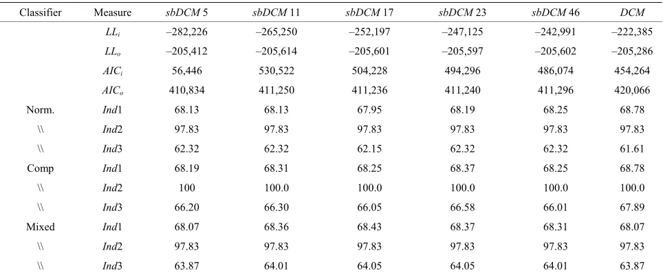
[image:5.595.196.494.87.200.2]Table 1. Classification results by varying cluster numbers and using matrix C.
Classifier Measure sbDCM 5 sbDCM 11 sbDCM 17 sbDCM 23 sbDCM 46 DCM
LLi –282,226 –265,250 –252,197 –247,125 –242,991 –222,385
LLo –205,412 –205,614 –205,601 –205,597 –205,602 –205,286
AICi 56,446 530,522 504,228 494,296 486,074 454,264
AICo 410,834 411,250 411,236 411,240 411,296 420,066
Norm. Ind1 68.13 68.13 67.95 68.19 68.25 68.78
\\ Ind2 97.83 97.83 97.83 97.83 97.83 97.83
\\ Ind3 62.32 62.32 62.15 62.32 62.32 61.61
Comp Ind1 68.19 68.31 68.25 68.37 68.25 68.78
\\ Ind2 100 100.0 100.0 100.0 100.0 100.0
\\ Ind3 66.20 66.30 66.05 66.58 66.01 67.89
Mixed Ind1 68.07 68.36 68.43 68.37 68.31 68.07
\\ Ind2 97.83 97.83 97.83 97.83 97.83 97.83
\\ Ind3 63.87 64.01 64.05 64.05 64.01 63.87
We now verify the goodness of the sbDCM models described in Section 3, to understand if we can insert latent topics into DCM by maintaining the burstiness and the same classification performance. Two kinds of ma- trixes have been used in the cluster procedure. One ma- trix contains the correlations among words C in the vo-
cabulary and another G is constructed by calculating the
Kruskal-Wallis index on the count matrix among words. The latter index g is defined as follows:
21 3 1
3
12 1
1
1
K i i i
p i i i
N n r N N
g
c c
N N
2
(15)
where ni is the number of sample data, N the total obser-
vation number of the k samples, k the number of samples to be compared and ri the mean rank of i-th group. The
denominator of the index g is a correction factor needed when tied data are present in the data set, where p is the number of recurring ranks and ci is the times the i-th rank
is repeated. The index g depends on the differences among the averages of the groups ri and the general
average. If the samples come from the same population or from populations with the same central tendency, the arithmetic averages of the ranks of each group
i ij j
r
r ni should be similar to each other and to the general average
N1 2
as well. The training dataset contains 2051 documents with a vocabulary of 4096 words for both approaches. The evaluation dataset (again the same for both models) contains 1686 documents which are distributed over 46 classes. In Tables 1 and 2we report the results from the two tests obtained respec- tively by matrixes C and G and by varying the number of
groups in the cluster. In the tables we indicate with LLin
the log-likelihood before the parameters updating and with LLout after the iteration procedure which is stopped
when the error = 10−10 is reached. The same with AIC
cin
and AICcout that is the corrected Akaike Information Cri-
terion (AICc) before and after the uploading. The indexes
Ind1, Ind2 and Ind3 have been described in Section 5.1. As we can see in the two Tables 1 and 2, the percent-
ages of correct classification (Ind1) are very close to the original ones with a parameter for each word (4096 pa- rameters). Of course they depend on the type of classifier employed during the classification step. Considering both
sbDCM and DCM, the differences produced by varying the number of groups are small. Moreover the AICc is
always better in the new approach then considering each word as a parameter (DCM model). In particular for what concerns the approach based on the correlation matrix C
(in Table 2) with 17 groups and on the Mixed classifier,
it can predict correctly the 68.43% of documents. The log-likelihood and the AICc indexes along groups are
quite similar, however the best value is obtained with 5 groups (respectively −205,412 and 410,834). Consider- ing again the approach based on the correlation matrix C,
we can conclude that, in terms of complexity expressed by the AIC index, the sbDCM approach whatever applied classifier is always better than the DCM. When we use matrix G (Table 2) the best classification performance is
for the complement classifier based on 23 groups, with a percentage of 68.72%, a log-likelihood of −204,604, the
AICc of 409,254. The best log-likelihood and AICc are for
cluster with 46 groups (respectively −204,362 and 408,816). Even if the sbDCM distribution based on matrix
G is not able to improve the classification performance of
Table 2. Classification results by varying cluster numbers and using matrix G.
Classifier Measure sbDCM 5 sbDCM 11 sbDCM 17 sbDCM 23 sbDCM 46 DCM
LLi –291,257 –283,294 –270,360 –266,453 –258,061 –222,385
LLo –205,912 –204,647 –204,600 –204,604 –204,362 –205,286
AICi 582,524 566,610 540,754 532,952 516,214 454,264
AICo 411,834 409,316 409,234 409,254 408,816 420,066
Norm. Ind1 67.83 67.71 67.47 67.42 67.65 67.66
\\ Ind2 97.83 97.83 97.83 97.83 97.83 97.83
\\ Ind3 62.02 61.73 61.45 61.43 61.55 61.61
Comp Ind1 67.95 68.66 68.55 68.72 68.60 68.78
\\ Ind2 100 100.0 100.0 100.0 100.0 100.0
\\ Ind3 67.95 68.09 68.05 68.29 68.05 67.89
Mixed Ind1 68.07 68.13 67.83 67.71 67.89 68.07
\\ Ind2 97.83 97.83 97.83 97.83 97.83 97.83
\\ Ind3 63.87 63.97 63.05 62.86 62.95 63.87
always better in terms of either AIC and log-likelihood indexes. Moreover, if we perform an asymptotic chi- squared test considering the two cases (matrixes
G and C) to decide whether the difference among log-
likelihoods (LL), with respect to DCM, are significant (i.e. the difference is statistically meaningful if the
2 test
1 2 is greater than 6), we can see from Tables 1 and 2 the test with matrix G has the best performance.
LL LL
Performance of the Semantic-Based Dirichlet Compound Multinomial with T Known in Advance
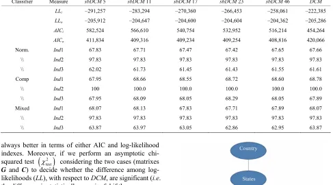
A different approach needs to be assessed when the number of available topic T is known in advance. In fact a text corpora could be enriched by several descriptions of treated topics according to the knowledge of field ex- perts. In more details, the analysis could be provided with a priori knowledge based on ontological schemas that describe the relations among concepts with regards to the general topics of the corpora. An ontology (from which an ontological schema is derived) is a formal rep- resentation of a set of concepts within a domain and the relationships between those concepts [16]. It provides a shared vocabulary, which can be used to model a domain, that is, the type of objects and/or concepts that exist, and their properties and relations. In Figure 3 we report an
example of graphical representation of an ontological schema. For example, if a text set deals with reputational risk management for corporate institutions, an ontology can be created on the basis of the four categories of problems (internal processes, people, systems and exter- nal events) defined by Basel II Accords.
Hence we can suppose that some specific sub-topics and key words, such as the possible causes of repute- tional losses, will be almost surely treated along the texts.
Figure 3. Example of ontological schema.
Thereby, the ontology structure provides the set of rela- tions among the concepts to which can be associated, by a field expert(s), a certain number of key words. Thus, we want to use the classes of a given ontology and the associated key words to define in advance the number T
inaccurate reporting by the media. A detailed and struc- tured analysis of what the media are saying is especially important because the media shape the perceptions and expectations of all the involved actors. Natural language processing technologies enable these services to scan a wide range of outlets, including newspapers, magazines, TV, radio, and blogs. In order to enable the application of the classification textual model sbDCM we have col- laborated with the Italian market leader company in fi- nancial and economic communication, Sole24ORE. Sole- 24ORE team provided us with a set of 870 articles about Alitalia, an Italian flight company, covering a period of one year (Sept 07-Sept 08).
The 80% of the articles are used to train the model and the remaining 20% to validate the process. The objective is to classify the articles on the basis of the reputation ontology in order to understand the argument treated in the articles. The ontology classes used for the classifica- tion are:
Identity: the perception that stakeholders have of the organization, person, product. It describes how the organization is perceived by the stakeholders.
Corporate Image: the “persona” of the organitation. Usually for companies visibly manifested by way of branding and the use of trademarks and involves the mission and the vision. It involves brand value. Integrity: personal inner sense of “wholeness” deriv-
ing from honesty and consistent uprightness of char- acter.
Quality: the achievement or excellence of an entity. Quality is sometimes certificated by a third part. Reliability: ability of a system to perform/maintain its
functions in routine and also in different hostile or/ and unexpected circumstances. It involves customer satisfaction and customer fidelitation.
Social Responsibility: social responsibility is a doc- trine that claims that an organization or individual has a responsibility to society. It involves foundation campaign and sustainability
Technical Innovation: the Introduction of new tech- nical products or services. Measure of the “RD orien- tation” of an organization (only for companies). Value For Money: the extent to which the utility of a
product or service justifies its price.
Those classes define the concept of reputation of a company. To link the ontology classes to the textual analysis we use a set of key words for each class of the reputation schema. Since the articles are in Italian, the key words are in Italian as well. For example the concept of “Reliability” involves customer satisfaction and cus- tomer fidelitation and is characterized by the following set of key words: affidabilità, fiducia, consumatori, ri- sorsa, organizzazione, commerciale, dinamicità, valore,
mercato. On the basis of these key words, we perform a
grouping analysis considering the 9 classes. From the clustering, we derive the matrix D. Empirical results show
good performance in terms of correct classification rate. We obtain that, given 171 articles, we correctly classify the 68% of them.
6. Conclusions
This contribution has shown how to enrich the DCM
model with a semantic extension. We also have proposed a method to insert latent topics within the “Dirichlet Compound Multinomial” (DCM) without losing the words “burstiness”: we call such a distribution “semantic- based Dirichlet Compound Multinomial” (sbDCM). The approaches assessed depend on the knowledge about the topics T. In fact there can be two alternative contexts: on one hand the topics are unknown in advanced, thus to be estimated on the basis of data at hand. On the other hand a text corpora could be enriched by several descriptions of treated topics according to the experience of the field expert(s). Specifically, the analysis can be empowered with a priori knowledge based on ontological schemas that describe the relations among concepts with regards to the general class argument of the corpora. In order to insert topics we create a new coefficient vector t for
each topic and later on we obtain the parameters as a linear combination of them. The methodology is based on a matrix D containing the degree of membership of
each word to a cluster (i.e. a topic) by using the cluster distance matrix. Then we split the words count vectors among latent topics and, by employing a fixed-point iteration, we generate the β coefficients representing the topics weights. In order to compare the two models DCM
and sbDCM we have employed a “Naive Bayes Classi- fier” based on the estimated distributions as shown in [13]. Several classifiers have been proposed and tested, and among them the best performance is obtained by means of the “mixed formula” and “CM10”. Moreover,
we run several tests to verify if the classification perfor- mance reached with an for each word (DCM) is main- tained or improved by the sbDCM.
Such an objective has been accomplished employing two different approaches. We propose two different me- thods to generate parameters, one based on the corre- lation among words C and the second based on the
Kruskal-Wallis index calculated on the words count matrix G. The results report that the test performances in
terms of misclassification rate are quite close to each other and to the performance reached by the DCM. However the sbDCM distribution is able to obtain better results in terms of AIC and log-likelihood especially in the case of matrix G. Concluding, by using matrix D to
cation performance and to follow the burstiness.
7. Acknowledgements
This work has been supported by MUSING 2006 con- tract number 027097, 2006-2010 and FIRB, 2006-2009). The paper is the result of the close collaboration between the authors, however the paper has been written by Paola Cerchiello under the supervision of Paolo Giudici.
REFERENCES
[1] S. Deerwester, S. Dumais, G. W. Furnas, T. K. Landauer and R. Harshman, “Indexing by Latent Semantic Analy- sis,” Journal of the American Society for Information Science, Vol. 41, No. 6, 1990, pp. 391-407.
doi:10.1002/(SICI)1097-4571(199009)41:6<391::AID-AS I1>3.0.CO;2-9
[2] T. Hofmann, “Probabilistic Latent Semantic Indexing,”
Proceedings of Special Interest Group on Information Retrieval,New York, 1999, pp. 50-57.
[3] D. M. Blei, A. Y. Ng and M. I. Jordan, “Latent Dirichlet Allocation,” Journal of Machine Learning Research, Vol. 3, 2003, pp. 993-1022.
[4] M. Girolami and A. Kaban, “On an Equivalence between PLSI and LDA,” Proceedings of Special Interest Group on Information Retrieval, New York, 2003, pp. 433-434. [5] D. M. Blei and J. D. Lafferty, “Correlated Topic Models,”
Advances in Neural Information Processing Systems, Vol. 18, 2006, pp. 1-47.
[6] D. Putthividhya, H. T. Attias and S. S. Nagarajan, “Inde- pendent Factor Topic Models,” Proceeding of Interna- tional Conference on Machine Learning, New York, 2009, pp. 833-840.
[7] J. E. Mosimann, “On the Compound Multinomial Distri- bution, the Multivariate B-Distribution, and Correlations among Proportions,” Biometrika, Vol. 49, No. 1-2, 1962, pp. 65-82.
[8] K. Sjolander, K. Karplus, M. Brown, R. Hughey, A. Krogh, I. S. Mian and D. Haussler, “Dirichlet Mixtures: A Method for Improving Detection of Weak but Signi- ficant Protein Sequence Homology,” Computer Applica- tions in the Biosciences, Vol. 12, No. 4, 1996, pp. 327- 345.
[9] D. J. C. Mackay and L. Peto, “A Hierarchical Dirichlet Language Model,” Natural Language Engineering, Vol. 1, No. 3, 1994, pp. 1-19.
[10] T. Minka, “Estimating a Dirichlet distribution,” Unpub- lished Paper, 2003.
http://research.microsoft.com/en-us/um/people/minka/pap ers/dirichlet/
[11] R. E. Madsen, D. Kauchak and C. Elkan, “Modeling Word Burstiness Using the Dirichlet Distribution,” Pro- ceeding of the 22nd International Conference on Machine Learning, New York, 2005, pp. 545-552.
[12] G. Doyle and C. Elkan, “Accounting for Burstiness in Topic Models,” Proceeding of International Conference on Machine Learning, New York, 2009, pp. 281-288. [13] J. D. M. Rennie, L. Shih, J. Teevan and D. R. Karge,
“Tackling the Poor Assumptions of Naive Bayes Text Classifier,” Proceeding of the 20th International Confer- ence on Machine Learning, Washington DC, 2003, 6 p. [14] A. P. Dempster, M. N. Laird and D. B. Rubin, “Maxi-
mum Likelihood from Incomplete Data via the EM Algo- rithm,” Journal of the Royal Statistical Society, Series B, Vol. 39, No. 1, 1977, pp. 1-38.
[15] D. Böhning, “The EM Algorithm with Gradient Function Update for Discrete Mixture with Know (Fixed) Number of Components,” Statistics and Computing, Vol. 13, No. 3, 2003, pp. 257-265. doi:10.1023/A:1024222817645 [16] S. Staab and R. Studer, “Handbook on Ontologies, Inter-
national Handbooks on Information Systems,” 2nd Edi- tion, Springer, Berlin, 2009.