Simulation mathematical model of expert system for working processes management

For the management of technological and work-ing processes in an agricultural enterprise, the only intensive method of decision based on the practical experiences is insufficient.

The high level of the enterprises equipment with ever more effective but also more expensive mecha-nisation requires that the decision on the concep-tion of agricultural enterprise equipment with mechanisation, machine purchase, and purposeful mechanisation utilisation should be supported by objectively determined arguments.

The expert system can be a source of these argu-ments specifying a suitable solution for concrete natural and production conditions in accordance with the given criteria. These criteria can be eco-nomical, energy or exploitation indicators.

Up to now, many programs and computing sys-tems have been developed in the Czech Republic, dealing more or less with the decision support in

technological and working processes planning, organisation, and management. they are mostly focused on partial problems such as, for example, the register (land and buildings, property shares, animals, etc.), animal nutrition, crops protection, agricultural practice measures etc.

The character of the expert system have the expert and information systems Agrokrom developed in the Agricultural Research Institute Kroměříž, Ltd. and techConsult consultancy system developed for sector of agricultural machine engineering.

The common feature of these two systems is the fact that they are based on the utilisation of the standards and norms which are often modified ac-cording to the production conditions characterised by operations difficulty or some other criteria.

Abroad, systems are used based on simulation mathematical modelling of particular operations within the working process for the selection of

supported by the Ministry of Agriculture of the Czech Republic, Project no. QF3200.

Simulation mathematical model of expert system

for working processes management

O. Syrový

_{, V. Podpěra}

1

_{Research Institute of Agricultural Engineering, Prague-Ruzyně, Czech Republic}

_{Anser, s.r.o., Prague, Czech Republic}

Abstract: The elementary simulation mathematical models presented in this article are related with the sub-system Crop production of the expert system for the decision support in technological and working processes management and their optimisation. Along with this sub-system, the expert system also involves the sub-systems Livestock produc-tion and Material handling which is further divided into the parts transport and storage. The boundary between the individual parts of the expert system is usually a short-term or long-term material storage. The relative individual sub-systems are mutually connected through the information flow. For each of the sub-sub-systems, specific simulation models are created. The simulation models in the expert system investigated replace the complex of general standards and norms used in other expert systems. The simulation models allow to take into consideration the concrete natural and production conditions (area, plots shape and inclination, soil type, transport routes length and surface, fertilisers doses, crops yields etc.) and also the technological systems utilised during the realisation of operations in working processes (technical, exploitation, energy, economical or energy means, attached vehicles, machines and equipment and method of their work) and the calculation of the parameters utilised. The simulation models also allow the creation of suitable working, and transport sets to choose their optimal variants for the given conditions. In comparison with the utilised standards and norms, the parameters computed through the simulation models significantly improve the data which represent the output from the expert system.

machines and equipment operating under concrete conditions of the respective agricultural enter-prise.

Kübler et al. (2006) are aware that, compared with industry agriculture is a retarded sector in the simulation models developing, and that in this sector no adequate simulation program has been developed. They have also found that the indus-trial solutions are not suitable for the utilisation in agriculture. sögaard and sörensen (2004) have developed a simulation model for optimal machine selection from the point of view of the lowest costs in the framework of the farm machine system. The output of this simulation model is a machines and energy means complex with optimal parameters for the given conditions.

The simulation and optimisation program simens (1998) serves to a similar purpose with the aim to

choose suitable agricultural mechanisation for the implementation of operations within the required period at the lowest costs possible.

The effort to equip economically the agricultural enterprises with mechanisation and to utilise it purposefully has led to the development of other programs (Audsley & Boyse 1974; Jannot & Cariol 1994; ekman 2000).

simulation mathematical modelling utilises the sub-system Crop production of the expert system for the support of decision in managing technologi-cal and working processes and their optimisation.

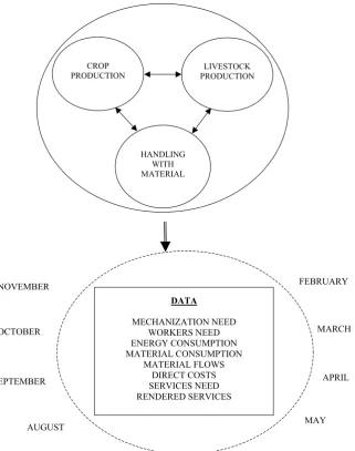
The work on this expert system is linked-besides the authors cited above – mainly with the works by Abrham (1995), Kavka (1997), and novák (1999). The expert system along with the sub-system Crop production includes the sub-systems Livestock pro-duction and Material handling (Figure 1) using their

DATA

MECHANIZATION NEED WORKERS NEED ENERGY CONSUMPTION MATERIAL CONSUMPTION

MATERIAL FLOWS DIRECT COSTS SERVICES NEED RENDERED SERVICES

FEBRUARY

MARCH

APRIL

MAY AUGUST

OCTOBER NOVEMBER

SEPTEMBER

LIVESTOCK PRODUCTION CROP

PRODUCTION

HANDLING WITH MATERIAL

own specific simulation mathematical models. The relative individual sub-systems are mutually linked through the information flow.

The objective of the expert system is to extend a wide scale of information enabling:

– to choose the optimal structure of the agricul-tural enterprise technical equipment,

– to optimise the working and transport sets for concrete operation conditions according to the criteria chosen in advance,

– to put together the most suitable working pro-cesses according to the given farming practices or zoo-technical requirements, and to evaluate them by the economical, energy, and exploitation parameters selected,

– to create the plan of the operational utilisation of machanisation (long-term, short-term),

– to specify the conditions and terms for the work realisation by services, or to determine, the free working capacity of the own technical means. The article is further focused on the method of the development of simulation models for the opera-tions utilised in the technological systems for the crop production.

METHOD

The simulation mathematical modelling is based on algorithms creation using the current theoretical knowledge, new knowledge obtained by analysis of the measurements results realised, own research activity, and other information acquired from pro-fessional literature.

on the basis of the algorithms created, the input values are specified for the subsequent computing programs of the expert system.

The simulation mathematical models utilised have to allow the computation of exploitation, energy, economical, or environmental parameters necessary for the decision on the implementation method for particular operations in the working processes of

agricultural products manufacturing under different natural and production conditions.

the models utilise the database giving infor-mation on mechanisation, agricultural practice requirements, natural and production conditions, up-to-date prices, and other factors influencing the operation and working process realisation.

The models have a dynamic character because they respond to the conditions change during the operations and working processes realisation as caused e.g. by the weather, yields achieved, fertilis-ers doses etc.

With regard to the computing processes complex-ity and their time requirements, it is necessary to utilise the computing equipment for the simulation model implementation.

RESULTS

Elementary mathematical simulation models

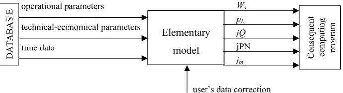
The elementary mathematical simulation models are a basis of the expert system. In these models utilising the input data acquired from the database (e.g. Plots, Livestock facilities, storage facilities, Model Working processes, Designed working processes, Crop rotation systems, operations, Plant, Materials, energy means, Machines and equipment, Attached vehicles, Agricul-tural enterprise milepost, etc) or adapted according to the updated conditions are calculated by the created algorithms and then transferred to other computing programmes as shown in Figure 2.

Optimisation criteria of the elementary model

The elementary model is based on the assumption that the requirements for the working processes and operations implementation resulting from the agricultural products production technologies can be fulfilled in optimal way on the basis of theoretical and practical knowledge.

operational parameters

technical-economical parameters

time data

user’s data correction Elementary

model

pL

jQ jPN jm

Ws

D

A

TA

B

A

S E

Consequent com

pu

tin

g

pr

og

ra

m

Figure 2. scheme of elementary simulation model connections in the expert system

The following criteria have been selected for op-timisation: work productivity, unit direct costs, and energy consumption related to the production unit.

As regards the work productivity, the labour saving is the main result of optimisation. The optimisation is important in the situations of working force short-age or workers high personal costs.

Usually the optimisation following the criterion of unit direct costs is of high importance and brings the working costs reduction.

In the case of fuels or other energy sources short-age or when their price is too high, the optimisation from the view of energy specific consumption plays more important role.

The elementary models are solved in such way that the resulting data correspond with the optimal levels of some of these criteria or with suitable relation-ships between them according to the user’s device.

Required performance determination

The first step is to specify the required total perfor-mance in operation or realisation on the plots P₁–P_n in such way as to maintain the terms of agricultural practices.

_{i=n (} Pn)

∑

Pi)

P_W

P(oi) = –––––––––––––––––––––––––––––– (|D_z – D_k| – D₀ + D_p) × T_d × k_sm × k_po where:

p_W

p (oi) – required total operation performance oi (h) P1 … Pn – plots

Si – Pi plot area (ha)

Dz – calendar day of agricultural practice time begin-ning (day)

Dk – calendar day of agricultural practice time finish (day)

D0 – number of non-working days within agricultural practice time

Dp – number of non-working days used for work Td – working day length (h)

ksm – shift coefficient kpo – weather coefficient

The computer will select the appropriate machine type from the mechanisation available for operation o_i realisation:

M_dt∈_Md where:

Mdt – sub-set of machine types suitable for the concrete operation

Md – set of machine types in the database a_tx∈_Mdt

where:

atx – machine type

If the appropriate machine type is not included in the available database or is not inserted into it dur-ing the creation of the enterprise conception of the mechanisation equipment, a machine is suggested from the set in which machines are characterised by the main exploitation parameter, e.g.

M_dt = {B₁ ... B_n} where:

B1 … Bn – machine working width (m)

to this parameter other data are adjoined that are necessary for the exploitation, energy, and economi-cal indicators determination economi-calculated on the basis of empiric equations generated according to the realised measurement (e.g. P_t = f (B,v), P_vh = f (ψ,v)), analysis of technical parameters (m_s = f (B)), or pur-chase price (e.g. C_p = f (B)).

C_p, m_s, P_t, P_vh, P_hy = f (B) where:

Cp – purchase price (CZK) ms – machine mass (kg)

Pt – necessary tensile output (kW) Pvh – input on Pto (kW)

Phy – input on hydraulic system (kW)

If the machine is not equipped by energy source, then this is determined according to the require-ment for the appropriate type (e.g. tractor 4K2, 4K4), and the necessary nominal output of its motor is calculated:

1 + δ P_vh P_hy 1

P_j=~

[

]

Pj – nominal output of energy means motor (kW) kP – coefficient of motor nominal output reserve (0.65–

0.80 by operation type)

Pf – output for energy means rolling resistance overcoming (kW)

Pα – output for energy means climbing overcoming (kW)

Pt – tensile output (kW)

Pvh – output withdrawal from Pto (kW)

Phy – output withdrawal from hydraulic equipment (kW)

δ – energy means driving wheels slippage

ε_vh – effectiveness of transmission from motor to Pto

ε_hy – effectiveness of transmission from motor to hydraulic equipment pump

while:

P_t, P_vh, P_hy = f (B, v_p,α_{, ko1 … kon ) (kW)} where:

B – machine working width (m) vp – working speed (km/h)

α – gradient (degree)

ko1 … kon – specific energy indicators of particular opera-tions (e.g. specific resistance, specific torque etc.).

Method of parameters determination representing the elementary model output

Exploitation parameters

Performance considered as an indicator expressing the intensity of technical means activity (or worker in working process) is calculated according to the algorithms for the individual types of operation. Generally, theoretical performance (W_t) is a function of some quantities presented.

W_t = f (B,ψ, v, ω, ω_a, m_m,T_t) (ha/h, t/h) where:

Wt – theoretical performance (ha/h, t/h)

ψ – row length mass (kg/m)

ω – plant yield (t/ha)

ω_a – application portion or seed stock amount (t/ha, kg/ha, l/ha)

mm – processed material amount (t, kg) Tt – working time (activity) (h, min)

note: T_t = time when machine performs the ac-tivity for which it is specified (ploughing, mowing etc). With this time corresponds also the theoretical performance (W_t).

The actual performance (Ws) is the main data for the work planning and managing and is determined according to:

W_s = W_t× k₀× k_sw× k_tp (ha/h, t/h) where:

Ws – real performance

ko – performance coefficient of turning ksw – performance coefficient of slope ktp – coefficient of technological intervals

The performance coefficient of turning (k_o) de-pends on the plot size and shape characterised by the ratio of the plot average length to its width and type of operation.

The coefficient of slope (k_sw) determines how the slope influences the theoretical performance in time in the dependence on the work method (e.g. bed, circular).

the coefficient of technological intervals (k_tp) expresses the time proportion (from total time) for repeating operations necessary for the machine activity, for example fertiliser and seed reception, harvested material unloading etc.

k_tp = f (V_z, ρ_{m, Ws, Tm)} where:

Vz – containers volume (m3)

ρ_m – material volume weight (kg/m3₎

Tm – handling time for containers filling or unloading (min)

The handling time (T_m) is given by: T_m = T_pm + T_p (min)

where:

Tpm – time of auxiliary handling operation (min) Tp – transfer time (min)

For the transfer time (T_p) is valid: T_p = f (W_pr, m_p)

where:

Wpr – performance of the transfer equipment (t/h, kg/min),

mp – weight of the transferred material (kg)

Work productivity (p_L) expresses the amount of the so called live work necessary per processed coefficient unit (ha, t) and is determined by the formula:

i_p

p_L = ––––– (h/ha, h/t) Ws

where:

ip – number of workers per operation

Energy parameters

The basic energy parameter is the consumption per mass unit of the manufactured product (Q_t) and is given by the sum of energy unit consumption in the working process operation (Q_tei) classified ac-cording to the energy type (e).

_n

Q_te =

∑

i=1

where:

Qte – energy specific consumption e (l/t, kWh/t, m3/t, kg/t) e – energy type (motor fuels, electricity, natural gas, solid

fuels etc)

The resulting energy specific consumption (Q_t) per the manufactured product unit consists of particular energy types consumptions [e(1) –e(m)]:

_{1=n 1=n 1=n}

Q_t =

∑

∑

∑

i=1 i=1 i=1

e(1) e(2) e(3)

When calculating the energy consumption in the working operations, the initial data is the hourly con-sumption (Q_h) generally expressed by the function:

Q_h= f (P_j,ε_{j, qεj) (l/h, kW/h, m}3_{/h, kg/h)}

where:

Qh – energy hourly consumption (l/h, kW)

Pj – motor nominal output (or other energy source) (kW)

ε_j – coefficient of nominal output utilisation

qεj – specific consumption at coefficient εj (g/kW, m3 per

kWh, kg/kWh)

Consumption per processed unit (ha, t) (Q_ha(t)) is given by the relationship:

Q_h

Q_ha(1) = ––––– (l/ha(t), kWh/ha(t), m3_{/ha(t), kg/ha(t))}

Wsha(t)

The calculations presented above are applicable for a machine or a machine set working within the plane ground. For the work on the slope, the results should be corrected by the slope energy coefficient k_sQ:

Q_h(α) = Q_h× k_sQ (l/h) where:

Qh(α) – hourly consumption during operation time on the

slope (α) (l/h)

ksQ – slope energy coefficient

Economical parameters

The basic economical indicators of the elementary model are the direct costs per unit of the product mass (jPN_t) similarly as for the energy consump-tion.

The direct costs per manufactured product unit (jPN_t) are given by the sum of the unit direct costs in the working process operations.

_n

jPN_t =

∑

where:

jPN_t – direct costs per production of product mass unit (CZK/t),

jPN_ti – direct costs per production of product mass unit in operation i

The initial data for the calculation of the direct costs per manufactured product mass unit (jPN_t)

are the costs per one hour of the mechanisation operational utilisation (jPN_h). These costs are given by the relationship:

jPN_t = jPN_he + jPN_hs (CZK/h) where:

jPNh – direct costs per one hour of the set operational utili-sation (CZK/h)

jPNe – direct costs per one hour of energy means opera-tional utilisation (CZK/h)

jPNs – direct costs per one hour of attached machine opera-tional utilisation (CZK/h)

The hourly direct costs (jPN_h) consist of fixed costs (constant) (jPNF_h) and variable costs (jPNV_h):

jPN_h = jPNF_h + jPNV_h (CZK/h) where:

jPNFh – direct fixed costs per one hour of operational utili-sation (CZK/h)

jPNVh – direct variable costs per one hour of operational utilisation (CZK/h)

If a machine is purchased for own financial means, the fixed hourly costs are influenced by the factors in the functional dependence:

jPNF_h = f (C_p, C_z, t_r, T_r, p, D_x, S_u,C_S) (CZK/h) where:

Cp – machine purchase price (CZK/h)

Cz – machine price after depreciation repayment (CZK) tr – machine depreciation time (year)

Tr – total operational time per 1 year (h) p – annual insurance rate (%)

Dx – taxes and fees (CZK/year) Su – storage area size (m2)

Cs – costs per storage area unit (CZK/m2)

If a machine is bought on loan, the fixed hourly costs depend on:

jPNF_h = f (C_p, u_p, u_i, t_s, t_r, T_r, p, D_x, S_u,C_S) (CZK/h) where:

up – loan interest rate (%)

ui – inflation average rate within the repayment time or leasing (%)

ts – repayment time (year)

If the machine is leased, then the fixed hourly costs are influenced by two factors:

jPNF_h = f (C_p, C_a, u_l, C_zl, t_l, t_r, T_r, p, D_x, S_u, C_s) (CZK/h) where:

The variable costs (jPNV_h) consist of costs of the mechanisation care, costs spent on energy and la-bour force according to the relationship:

jPNV_h = jPNO_h + jPNE_h + JPNP_h (CZK/h) where:

jPNVh – variable costs per one hour of the machine opera-tional utilisation (CZK/h)

jPNOh – costs of the machine care related to one hour of the machine operation (CZK/h)

jPNEh – costs of consumed energy related to one hour of the machine operation (CZK/h)

jPNPh – hourly costs of the labour force (CZK/h)

The unit costs of the machine care (jPNO_h) depend on the factors:

for energy means or machines equipped with energy source:

jPNO_h = f (C_p, C_z, t_r, m_ol, Q_hr) where:

mol – coefficient of the care related to energy consumed during one year (e.g.103 _{l of motor Diesel, 10}3 _kWh

of electricity etc.)

Qhr – energy annual consumption (l, kwh, m3) for machines without energy source:

jPNO_h = f (C_p, C_z, t_r, T_r, m_oh) (CZK/h) where:

moh – coefficient of care related to the number of hours of the operational utilisation during one year

The unit direct costs of consumed energy depend on: jPNE_h = f (Q_h, C_e) (CZK/h)

where:

Ce – energy price (CZK/l , CZK/kWh, CZK/m3)

The unit direct cost of the labour force (jPNP_h) is influenced by the factors:

jPNP_h = f (i_p, C_M, C_D, k_p, C_o) where:

ip – number of workers included into qualification classes

Cm – hourly wage rate in appropriate qualification class (CZK/h)

CD – additional hourly costs (CZK/h)

kp – coefficient of employer contribution to social and medical insurance

Co – other costs of the labour force related to worked off hour (CZK/h)

The costs on processed unit (ha, t) are given by the relationship:

jPN_h jPN_ha(t) =––––– Wsha(t)

Related programs

Program of operation implementation on plot

This program is aimed at the working set deter-mination (self-propelled machines) suitable for working operation implementation according to the selected criteria (lowest costs, lowest work productivity).

Following the data from the elementary model, the set is chosen with the best parameters according to the selected criterion. If that set performance (W_si) is lower than the total performance required for the operation implementation (p_W

p) on plot Px: p_W

p> Wsi=1

then the other most suitable set is persued up to the fulfilment of the following condition:

_n p_W

1 ≤

∑

Further, the monitored data are summarised on the plot P_x,_.i.e.:

_n

∑

where:

ThEi – energy means i work need (h) ThSi – machine i work need(h) ThLi – workers i labour need (h) ThE – energy means total work need (h) ThS – machine total work need (h) ThL – workers total labour need (h)

n

∑

where:

Qsei – energy consumption e by set e (l) PNi – direct costs of the set operation i (CZK) msi – material consumption by set i (t, kg, l) mpi – mass of material processed withset i Qse – energy total consumption j (l) PN – total direct costs (CZK)

ms – total consumption of material (CZK) mp – total mass of processed material

Program of determination of time periods of working operation on plot

This program allocates the data related to particu-lar operations of the selected working procedure to the chosen periods (day, week, decades) during the year (τ_rx):

– workers labour need (L_hL), – energy j consumption (Q_se), – direct costs (PN),

– material consumption (m_s), – processed material mass (m_p).

Program of time period summarisation

This program summarises the above presented data specified for particular operations and plots to acquire the total overview about their utilisation during a year.

Through the summarisation the need of services is also specified as well as the machine fleet free capacities as the basis for these services offer.

on the basis of these data, the user can suggest corrections and changes (e.g. in the set composition, operations terms, progress in operations implemen-tation on particular plots, in working processes etc.) or can decide on services exploitation from other organisations.

DISCUSSION AND CONCLUSIONS

The elementary simulation mathematical models of working processes in agricultural products manu-facturing give information enabling to optimise the production process according to the criteria given in advance. These can be connected with the solution of economical problems (production costs reduction) and energy problems (energy consumption reduc-tion), with the exploitation of the utilised mechani-sation (work productivity increasing) but also with the effort to reduce the unfavourable impacts of production activities on the farm land and environ-ment (reduction of contact pressure of energy means travel mechanism on the farm land, reduction of air burden with emissions, noise reduction, etc.) or with the solution of other problems in accordance with the selected criteria.

The simulation mathematical models presented are related with the sub-system Crop production of the expert system for the decision support in technological and working processes management and their optimisation. Along with this sub-system the expert system also involves the sub-systems Livestock production and Material handling which is further divided into parts transport and storage. The boundary between the individual parts of the expert system is usually the short-term or long-term material storage. The individual sub-systems are mutually connected through the information flow. For each of the sub-systems, specific simulation models are created. The simulation models in the expert system investigated replace the complex of

general standards and norms used in other expert systems.

The simulation models allow to take into con-sideration the concrete natural and production conditions (area, shape and inclination of plots, soil type, transport routes length and surface, fertili-sers doses, crops yields etc.) and also technological systems utilised during the realisation of the opera-tions in working processes (technical, exploitation, energy, environmental parameters of energy means, attached vehicles, machines and equipment and methods of their work) and during the calculation of the utilised parameters. The simulation models also allow the creation of suitable working and transport sets to choose their optimal variants for the given conditions. the parameters computed through the simulation models significantly improve the data which represent the output from the expert system in comparison with the utilised standards and norms.

the expert system is destined for some stages of utilisation. For agricultural enterprise management (creates work plans, specifies operational utilisa-tion of mechanisautilisa-tion, number of workers, costs drawing, energy and material consumption, speci-fies requirements for work realised by services and creates basis for own activities offer to other enter-prises, optimises agricultural enterprise equipment by agricultural mechanisation, specifies suitable working and transport sets for the conditions of agricultural enterprise), for the management of ma-chine services enterprise for agricultural primary production (simulation of conditions in which the enterprise operates, the same basis for manage-ment is obtained as at the agricultural enterprise), for state administration organs (simulation of general natural and production conditions, e.g. according to the production areas the information can be obtained about the assumed direct costs of agricultural products manufacturing, number of workers, energy and material consumption, etc., of different levels of technical equipment of agri-cultural enterprises and the machine-technological systems utilised).

References

Abrham Z. (1995): Determination and economical evalu-ation of costs for mechanized operevalu-ations in agriculture. Ústav zemědělských a potravinářských informací, Praha. (in Czech)

program. Journal of Agricultural engineering Research, 29: 141–149.

ekman s. (2000): tillage system selection? A mathemati-cal programming model incorporating weather vari-ability. Journal of Agricultural engineering Research, 77: 267–276.

Jannot P., Cariol D. (1994): Linear programming as an aid to decision – making for investments in farm equipment for arable farms. Journal of Agricultural engineering Re-search, 59: 173–179.

Kavka M. (1997): Utilization of agrarian mechanization under market economy conditions. Ústav zemědělských a potravinářských informací, Praha. (in Czech)

Kübler s., Fechner W., Wendt K., Pickel P. (2006): entwicklung landwirtschaftlicher simulationssoftware. Landtechnik, 61: 20–21.

novák J. (1999): Contribution for payment and its utili-zation in both over-enterprise and enterprise practice. Ústav zemědělských a potravinářských informací, Praha. (in Czech)

simens J.C. (1998): Agricultural systems modelling and simulation. In: Field Machinery selection Using simulation and optimization. the University of Florida, Gainesville, 543–566.

sögaard H.t., sörensen C.G. (2004): A model for optimal selection of machinery sizes within the farm machinery system. Biosystems engineering, 89: 13–28.

Received for publication March 19, 2008 Accepted after corrections June 13, 2008

Corresponding author:

Ing. otakar syrový, Csc.,Výzkumný ústav zemědělské techniky, v.v.i., Drnovská 507, 161 01 Praha 6-Ruzyně, Česká republika

tel.: + 420 233 022 277, fax: + 420 233 312 507, e-mail: [email protected]

Abstrakt

syrový o., Podpěra V. (2009): Simulační matematické modely expertního systému pro řízení pracovních postupů. Res. Agr. eng., 55: 1–9.

elementární simulační matematické modely uvedené v článku jsou základem subsystému Rostlinná výroba – expert-ního systému pro podporu rozhodování při řízení technologických a pracovních procesů a jejich optimalizaci. Vedle tohoto subsystému jsou součástí expertního systému další subsystémy a to Živočišná výroba a Manipulace s mate-riálem, která se dále člení na části Doprava a skladování. Relativně samostatné subsystémy jsou vzájemně propoje-ny tokem informací. Pro každý subsystém jsou vypracovápropoje-ny specifické elementární simulační matematické mode-ly. simulační matematické modely v řešeném expertním systémů nahrazují soulad standardů a normativů, které se používají v obdobných expertních systémech. simulační matematické modely umožňují při výpočtech použitých ukazatelů brát zřetel jak na konkrétní přírodní a výrobní podmínky (výměra, tvar a svažitost pozemků, druh půdy, délku a povrch dopravních tras, dávku hnojiv, výnosy plodin apod.), tak i na použité technologické systémy (na technické, exploatační, energetické popř. environmentální ekonomické parametry energetických prostředků, přípoj-ných vozidel, strojů a zařízení a na způsob jejich práce). simulační modely také dovolují vytvářet vhodné pracovní a dopravní soupravy a volit jejich optimální varianty.simulační modely, oproti používaným standardům a normati-vům, významně zpřesňují údaje, které jsou výstupem z expertních systémů.