works (WBSN) compete for occupation of a number of frequency channels. Each channel can host at most one WBSN with satisfactory performance and WBSNs have the ability to change their operating channel, subject to the constraint that they can only monitor the performance or occupancy of their current channel but not of any other channel. We consider a number of randomized schemes for changing the fre-quency channels and present and evaluate Markov chain models for these, building on a “balls-in-bins” approach.
2 Andreas Willig Noname manuscript No.
(will be inserted by the editor)
Autonomous Allocation of Wireless Body-Sensor Networks
to Frequency Channels: Modeling with Repeated
“Balls-In-Bins” Experiments
Andreas Willig
the date of receipt and acceptance should be inserted later
1 Introduction
Wireless body sensor networks (WBSNs) have received lots of interest recently, be-cause they enable a range of applications in health and well-being [21], [6], [2], [34]. A number of technologies are considered for WBSNs, including the IEEE 802.15.4 [20] and IEEE 802.15.6 [19] standards. On the physical layer the IEEE 802.15.4 standard specifies three different frequency bands that can be used. Two of these are sub-divided into a number of frequency channels, and a WBSN at any time operates on only one of these channels. For example, the popular 2.4 GHz ISM range is sub-divided into 16 channels of 5 MHz width each. Similarly, the IEEE 802.15.6 standard supports a number of different frequency ranges in its narrowband physical layer, and all these frequency ranges are sub-divided into several channels (79 in the 2.4 GHz range). In both standards it is foreseen that a WBSN does not routinely hop over the channels but rather picks a channel and stays there.
We consider situations where several independent WBSNs are forced to operate in close proximity to each other (for example when many people congregate in a sports stadium) and have to share wireless resources. In particular, each WBSN must decide on a frequency channel on which it operates. To detect co-location with other WBSNs in the same channel, we assume that WBSNs have the capability to mon-itor their own performance, e.g. packet loss rate, delay, number of retransmissions or other relevant indicators. In response to performance degradations from compet-ing WBSNs, a WBSN can theoretically adjust a wide range of operational parame-ters (e.g. transmit power or data generation rate), but in this paper we focus on how WBSNs can make autonomous decisions about their frequency channel. In previous work we have demonstrated how such a capability can be practically implemented for IEEE 802.15.4 [40], [26].
We consider an abstract version of this setting and seek insights into the opera-tion and performance of simple probabilistic strategies by which individual WBSNs
decide autonomously when to switch to another channel, with the goal of quickly set-tling into a channel assignment satisfying the communications needs of the involved WBSNs. Suppose we are givenN different channels andKdifferent WBSNs. For simplicity we make the assumption that one channel can satisfy the communication needs of no more than one WBSN. When two or more WBSNs are present on a chan-nel (which we refer to as acollision) then all WBSNs will experience insufficient transmission quality (please note that the precise definition of transmission quality does not matter for our purposes). We assume that all colliding WBSNs notice this immediately and might subsequently decide to jump to another channel. Under these assumptions there are two fundamentally different cases to consider:
– WhenK ≤N, i.e. the number of WBSNs does not exceed the number of chan-nels, then it is clearly possible to find an allocation of WBSNs to channels that satisfies everyone – we will refer to such an allocation as a “noncolliding state”. A key performance metric is the average time to reach a non-colliding state.
– WhenK > N then no non-colliding state exists and the choice of performance measure is not so clear-cut. Ideally, there should also be some degree of fair-ness among the WBSNs, i.e. each WBSN should experience satisfactory channel quality at least for some fraction of time and should be able to communicate suc-cessfully fairly frequently. The problem then becomes similar to load-balancing problems.
The main focus of this paper is on the caseK ≤ N, and we develop and analyse algorithms aiming to minimize the average time until there are no collisions. We will also assess the performance of one of these algorithms in the caseK > N.
1.1 Contributions
We make four main contributions:
– We investigate a simple probabilistic algorithm, called therestrained-jumping scheme(RJS), in which a colliding WBSN jumps with a pre-specified probability
– The RJS algorithm does not require individual WBSNs to keep any state besides knowing the value of the jumping probabilityp. We propose a modified proba-bilistic algorithm calledRJS-OB(where OB stands for “one-bit”), in which each WBSN uses a state of one additional bit to modify its jumping probability when colliding with other WBSNs, to the effect that a WBSN which has found a free channel and has “settled” there will now show some reluctance to leave by adopt-ing a smaller jumpadopt-ing probability. We evaluate the performance of this algorithm through simulations for the caseK≤Nand show that it offers substantially re-duced times to reach non-colliding states as compared to the best RJS algorithm. To the best of our knowledge, the RJS-OB algorithm is new.
– We consider a corner case of the RJS-OB scheme called thesticky scheme, in which WBSNs that have occupied a channel for at least one time slot as a sole occupant refuse to ever jump away from it. ForK ≤N this scheme shows the best performance in terms of the average time to reach a non-colliding state, but forK > N it will be very unfair, allowing some WBSNs to grab a slot forever while the other ones have to jump around eternally. We develop a Markov model for this scheme (valid forK ≤N), establish some of its properties and provide numerical and simulation-based evidence that the average time to reach a non-colliding state increases only in an approximately linear fashion for largeN and
K ≤N. The sticky scheme thus substantially outperforms the RJS-OB and the best possible RJS scheme.
– While being designed to minimize the hitting time in the caseK ≤N, the RJS-OB scheme is also applicable when K > N. We consider its fairness and the percentage of successful slots for a range of its parameters, and argue that it can be configured in a way that limits unfairness and approaches the performance of a pure balls-in-bins allocation (i.e. an allocation where each ball picks its bin independently and uniformly) from above, whereas by adding some unfairness the RJS-OB scheme achieves better performance.
We argue that the developed models and algorithms are of significant practical in-terest and are attractive candidates for the considered scenario. The algorithms have some key advantages:
– They are completely distributed and require no communication between WBSNs.
– They are guaranteed to converge to a non-colliding state with probability one, assuming it exists (i.e.K≤Nholds), and we hypothesize that the sticky scheme asymptotically achieves this on average in a time linear inN.
protocols for graceful release of channels or for periodic re-acquisition of a channel. It appears likely that these additions require changes to the existing WBSN technologies (IEEE 802.15.4, IEEE 802.15.6), which is generally undesirable and might lead to interoperability problems.
On the theoretical side this paper contributes novel and exact abstract Markovian models for discrete-time (or round-based) repeated balls-in-bin models, which may also have applications in other fields of networking and distributed systems.
1.2 Related Work
Broadly, this paper is in the area of frequency or channel allocation for wireless net-works [7], [1]. In contrast to technologies like Bluetooth or the TSCH variant of IEEE 802.15.4 which apply frequency hopping all the time, the IEEE 802.15.6 stan-dard and the original IEEE 802.15.4 stanstan-dard (on which ZigBee is based) follow a model in which a WBSN will normally stay on the same channel throughout, unless higher layers make a decision to switch the channel. This is the model considered in this paper. The IEEE 802.15.6 standard [19] foresees a mechanism for channel-hopping, for the IEEE 802.15.4 standard such a mechanism has been described in [40]. Here, a WBSN observes its own performance and switches to another frequency channel in the 2.4 GHz band when the performance is unsatisfactory. The perfor-mance evaluation has been carried out for the case of external interference coming from WiFi interferers. A similar mechanism has been used in [26] for a scenario in which many co-located IEEE 802.15.4 networks have to share the same channel re-sources in the 2.4 GHz band and create so-called internal interference to each other. The results show that with autonomous channel adaptation a better utilization can be achieved and more WBSNs achieve satisfactory packet loss performance. It should be noted that frequency adaptation is not the only mechanism that has been considered to deal with internal performance. Other proposals suggest to adapt the parameters of the MAC protocol, for example the beacon and superframe order in IEEE 802.15.4 [33], [28], [32], or the parameters of the backoff process [36], [8]. Power adapta-tion has been considered in [39]. Other frequency allocaadapta-tion or adaptaadapta-tion algorithms are for example discussed [10] (a follow-up on [9]), which integrates frequency al-location with adjustment of transmission phases, and [31], [13], which propose an algorithm somewhat similar to the RJS algorithm, but with jumping probabilities that depend on the number of networks or nodes in the same channel. In our paper we only assume that an individual WBSN can tell whether it has sufficient channel quality or not, but it is not able to estimate the number of contenders, as that would require extra measurement procedures.
allbins and, if it jumps, to pick only one of the bins which are either free or colliding. For example, in the PRMA protocol time is sub-divided into superframes, which are then further sub-divided into time-slots. A station picks a time slot for transmission, and if it was the only transmitter in this slot, it will properly receive an acknowledg-ment. This can be observed by all other stations, which will then avoid this time slot until it becomes free again. Decisions on a time slot to pick are made at the end of a superframe when all time slots have been observed. In the schemes considered in this paper, however, a node can always only observe its own bin and has no information at all about the other bins.
Balls-in-Bins problems (also often referred to as random allocations) have been widely considered in probability theory, see for example the monographs [16], [18]. In particular, results are available for the distributions of the minimum and maximum occupancy of an urn [14]. They also have found applications in wireless channel al-location problems [7], [1], load balancing problems for cache servers or cloud com-puting in the Internet [37], [35], [3], in task allocation problems in crowdsourcing applications [23], or in the analysis of hashing schemes [11]. In many of these papers an assumption is made that a “ball” looking for a “bin” has a chance to inspect the contents of a number of randomly chosen bins before making any decision, and then it will pick the most favorable (e.g. the least loaded) bin of these. This differs from our setting in that we assume that a WBSN can only observe its current channel and not any others.
In this paper we particularly consider the case of repeated balls-in-bins experi-ments, in which a random subset of colliding balls jumps again, until a non-colliding allocation has been reached, making the system under consideration an example of a (discrete-time) interacting particle system [24]. However, our setting is different from the standard models considered in the interacting particle systems literature (e.g. ex-clusion processes, contact processes, voter models), and to the best of our knowledge this kind of processes and their convergence time towards non-colliding states have not been widely considered in the literature.
1.3 Paper Overview
2K ≤N: An Exact Model for RJS
We assume slotted time. At the beginning of a time slot each WBSN checks whether it collides with one or more other WBSNs in the same channel. If not, the WBSN stays on the current channel for the remainder of the time slot. Otherwise, the WBSN – independently of other WBSNs – jumps out of its current channel with probability
p ∈ (0,1) and picks any of the remainingN −1 channels with equal probability. The jumping will happen shortly before the end of the current time slot. We will refer topas thejumping probability. For convenience, from here on we will leave the specifics of WBSNs behind and adopt a more combinatorial model and language. We will refer to the different channels asbinsand to the WBSNs asballs. Therefore, our system is related to random allocations [16], [14], but the presence of collisions, the introduction of a jumping probability, and the repeated throwing of a subset of the balls (the colliding ones) gives it unique characteristics.
The state space in the exact model captures all possible allocations ofKballs to
Nbins, it is given by
SN,K=
(
s= (s1, . . . , sN) :si∈N0, N
X
i=1
si=K
) ,
i.e. the set of allN-vectors(s1, . . . , sN)with non-negative integer entries summing up toK. In such a state the componentsiindicates the number of balls in bini. From simple combinatorial considerations the size of the state space is
|SN,K|=
N K
=(N+K−1)!
(N−1)!·K! (1)
We partition the state space into two different classes of states: into non-colliding states
NN,K={s∈ SN,K:si≤1, i= 1, .., N}
(where for all statess = (s1, . . . , sN)in this class we havesi ≤ 1for alli) and colliding statesCN,K=SN,K\ NN,K. ForK≤Nthe set of non-colliding states is nonempty and has size
|NN,K|=
N K
(2)
For the calculation of the state transition probabilities it is convenient to introduce the notion of thetypeof a states = (s1, . . . , sN). This type is given by listing the numbers s1, . . . , sN sorted in decreasing magnitude and dropping the zeros at the end (if any). The type of a statesis denoted by T(s). As an example, the type of state s = (0,2,3,7,1,0,0,0) is T(s) = (7,3,2,1). Furthermore, we denote by
T(s) ={t∈ SN,K:T(t) =T(s)}the set of all states that have the same type as states.
when starting from any of the colliding states (this is also known as ahitting time, see [29, Sec. 1.3]). The number of equations is given by|SN,K| − |NN,K|and grows rather quickly inNandK(compare Equations (1) and (2)). We discuss in Appendix A how one can reduce the system size substantially. The solutions for the hitting time in general depend on the starting state as well as on the parameterp.
2.1 Transition Probabilities
We consider the Markov chain governing the movements of the balls in the bins and derive its probability transition matrixP =P(N, K, p) = [[p(t|s)]]s,t∈S
N,K, with entryp(t|s)being the probability to go from statesto statet.
Our aim is to find the probability of transitioning from one states= (s1, . . . , sN)∈
SN,Kto a given successor statet= (t1, . . . , tN)∈ SN,K. Since we assume that for any non-colliding states∈ NN,Kthere are no further movements, we clearly have fors∈ NN,Kthat:
p(t|s) =
1 : s=t 0 : otherwise and hence the non-colliding states are absorbing.
Now consider a colliding start states= (s1, . . . , sN)∈ CN,K. In this statesthere is at least one binifor whichsi >1. Without loss of generality we assume for the following discussion that the colliding bins are the first ones, followed by the non-colliding bins, i.e. there exists somek∗ ∈ {1, . . . , N}such thats
i > 1fori ≤k∗ andsi ≤1fori > k∗. In general, there may be many different movements of balls that might lead from statesto statet. Consider as an exampleN = 10andK= 8, where the possible movements to get from states= (0,3,0,1,0,0,4,0,0,0)to state t= (0,3,0,1,1,1,2,0,0,0)include the following:
– (2,5)(2,6)(2,7)(7,2)(7,2)(7,2), where a pair(i, j)indicates that a ball is moved from binito binj
– (7,5)(7,6)
– (7,2)(7,2)(2,5)(2,6)
– (7,2)(7,5)(2,6).
Note that all these different movements in general occur with different probabilities.
To calculate the overall transition probability, we decompose states= (s1, . . . , sk∗, sk∗+1, . . . , sN) intok∗+ 1different vectors, namelys1 = (s1,0,0, . . . ,0),s2 = (0, s2,0, . . . ,0),
. . . ,sk∗ = (0, . . . ,0, sk∗,0. . . ,0)(which we will call the pure states) and the resid-ualsr= (0, . . . ,0, sk∗+1, . . . , sN)in which each entry is≤1. Below we show how to calculate the transition probability from a pure state (say,s1) to any of its possible successor states, the set of which we denote asPi for pure statesi. With this no-tation, and using standard vector addition, we can express the transition probability from statestotas
p(t|s) = X t1∈P1,...,tk∗∈Pk∗
t1+...+tk∗+sr=t
where we have used that the jumping decisions made by different balls are indepen-dent. The transition probability from one of the pure states, say states1= (s1,0, . . . ,0) to one of its successor states, sayt1= (t1, . . . , tN)witht1+. . .+tN =s1, is given by:
p(t1|s1) = (1−p)t1·
p N−1
s1−t1
·
s1
t1, . . . , tN
(4)
where
n
k1, . . . , kN
= n!
k1!·. . .·kN!
is the multinomial coefficient. The first factor accounts for the t1 balls that have opted to stay within their current bin (with probability1−peach). The second term accounts for thes1−t1balls that have opted to jump (with probabilityp) to one of theN −1other bins (with each other bin having the same probability). The final multinomial coefficient counts the number of ways in whichs1distinguishable balls can be partitioned so that the first bin getst1balls, the second bin getst2balls and so on.
Please note that in the caseK≤N (i.e. at most as many balls as bins) the set of non-colliding states is non-empty, and that these states are absorbing. Furthermore, forp∈(0,1)all the colliding states are transient states, since they jump with positive probability into one of the noncolliding states from which they never come back. This implies that the Markov chain will with probability one reach one of the non-colliding states when started in any state [29].
2.2 Hitting Time Calculation
We proceed towards the calculation of the key performance metric for the caseK≤ N, which is the average number of steps (or the average time) to reach a non-colliding state t ∈ NN,K from some starting states ∈ CN,K. This time is also known as ahitting time, in our case for the set of non-colliding states. It is well known that the vector(ks:s∈ SN,K)of hitting times for all start statess ∈ SN,K solves the following system of linear equations ([29, Thm. 1.3.5]):
ks= 0 :s∈ NN,K (5)
ks= 1 +Pt∈CN,Kp(t|s)·kt:s∈ CN,K (6) Note that [29, Thm. 1.3.5] and [29, Thm. 4.2.3] imply that the solution to Equa-tions (5) and (6) exists, is unique and non-negative. Unfortunately, even for small to moderate values ofN andKthe size of this linear equation system grows quickly, which makes it hard to solve in practice. For example, forN = 15andK= 10the full system comprises of|S15,10| − |N15,10| = 1,961,256−3,003 = 1,958,253 unknowns.
possible types forK balls corresponds to the number of partitions of an integerK, for which an explicit expression is not known (see [14, Sect. I.3.1], see also OEIS A0000411), but asymptotically (for largeK) this number is approximately [14, Sect. I.3.1]:
1
4K√3 ·exp π
r
2K
3
!
(7)
In our example withN = 15andK = 10the system size reduces to 41 unknowns (see Appendix A). However, this method does not eliminate the calculation of all transition probabilities according to Equation 3, which remains a limiting factor.
2.3 Numerical Results
For the case ofK = 2it is straightforward to establish and solve the system (5) for a generic value of the jumping probabilityp. There is only one colliding type, the hitting times for all colliding states are identical, and it is possible to find the value of
pwhich minimizes the common hitting time as
p∗= N−1
N
so that the common hitting time becomes
h(p∗) = N
N−1
Note that for larger values ofN (i.e. more empty bins) the optimal jumping proba-bilityp∗increases – i.e. the more free bins there are, the more aggressively colliding nodes should jump. However, the caseK = 2is deceivingly simple and already for
K = 3new phenomena occur. First, the average hitting time is in general different for two colliding states of types(3)and(2,1). In particular, for the considered values of N the best achievable hitting time for type (3)is generally larger than the best achievable hitting time for type(2,1). Secondly, for both types (3)and(2,1) the optimal jumping probability increases asNincreases, with more free space it makes sense to jump more aggressively. But for each considered value ofN, the optimal jumping probability for type(3)is smaller than for type(2,1), i.e. balls from more crowded bins should jump less aggressively than balls from less crowded bins. Note that forK≥3we have not been able to find closed-form expressions for the optimal jumping probability, as it involves finding roots of polynomials of fifth and higher degree [12, Chap˙14].
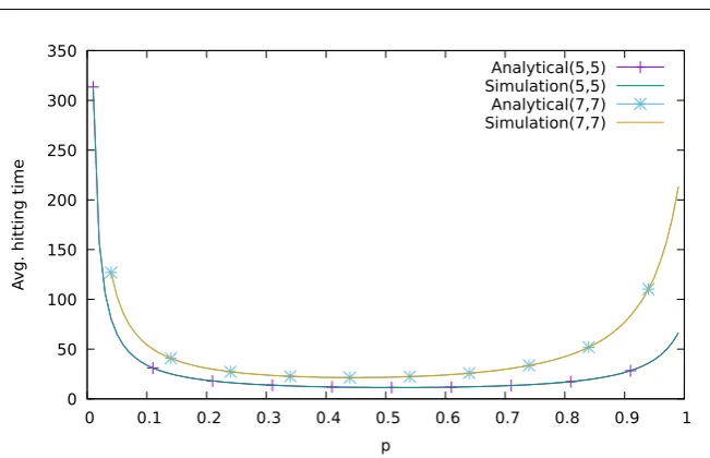
In Figure 1 we show results for the two casesN =K = 5andN =K= 7, for the jumping probabilitypranging from 0.04 to 0.99 in steps of 0.01, and a starting state where all balls are placed in the same bin. The figure shows the average hitting time versusp, obtained both numerically from the Markov model, and from running a
0 50 100 150 200 250 300 350
0 0.1 0.2 0.3 0.4 0.5 0.6 0.7 0.8 0.9 1
A
vg. hitting time
p
Analytical(5,5) Simulation(5,5) Analytical(7,7) Simulation(7,7)
Fig. 1 Hitting times for varyingpfor a system withN =K= 5andN=K= 7(all balls start in the same bin).
custom-made Monte-Carlo simulator.2In the simulation, we have carried out 20,000
replications of the experiment for each value ofp, and in the figure we report the average of these. There are two important conclusions: the first is that simulation and the analytical model show excellent agreement (the curves for the simulation and analytical results for the same value ofN =Koverlap perfectly), which enhances trust in the validity of either of these. Secondly, it can be seen that the actual choice ofphas a substantial impact, with average hitting times forN = K = 5ranging from a few hundreds of time steps (for smallp) down to a minimum of≈11.4time steps, similarly forN =K= 7.
In Figure 2(a) we show for varying N andK ∈ {N, N −1} and for diffent choices of the type of initial state the optimal jumping probabilities, i.e. the proba-bilities that achieve the smallest average hitting times. These probaproba-bilities have been obtained numerically from the Markov model by considering allpbetween 0.01 and 0.99 with a spacing of 0.01. In Figure 2(b) we show the resulting best hitting times. The following observations hold:
– When increasingN while keeping the differenceN −K fixed, the optimal p
decreases with increasing value of N, while the resulting optimal hitting time increases withN (andK) at a superlinear rate.
2 The simulator has been written in the Haskell programming language. Its operation is conceptually
[image:11.595.76.402.76.286.2]0.4 0.45 0.5 0.55 0.6 0.65 0.7
3 4 5 6 7 8
Best jumping pr
obability
N
N=K, Type=(K) N=K, Type=(K-1,1) K=N-1, Type=(K-1)
(a) Best jumping probabilities
0 5 10 15 20 25 30
3 4 5 6 7 8
Best hitting time
N
N=K, Type=(K) N=K, Type=(K-1,1) K=N-1, Type=(K-1)
(b) Best hitting times
Fig. 2 Best jumping probabilities / hitting times for varyingN,K, different start types
– Clearly the optimalpdepends on this differenceN−K, andpshould be chosen larger as this difference increases.
– From Figure 2(b), the best hitting time for the type(K)is generally slightly larger than the best hitting time for type(K−1,1). We hypothesize that generally the type(K)has the worst hitting time of all types and can thus be regarded as a “worst-case” type, but for increasingKthis difference vanishes.
– We can also confirm the previously observed trend that for a givenN the hitting times increase withK.
Unfortunately, besides identifying these trends, the complexity of the Markov model for RJS makes it very difficult to find a closed-form expression for the optimal value ofpfor givenNandK.
50 100 150 200 250 300
5 10 15 20 25
A
vg. hitting time
N=K
0.1 0.15 0.2 0.25 0.3
[image:12.595.77.404.68.197.2] [image:12.595.79.396.426.615.2]Max. bin occupation # Occurences Percentage
2 14,568 84.06
3 2,666 15.38
4 65 0.38
5 3 0.02
6 3 0.02
[image:13.595.104.337.85.160.2]≥7 26 0.15
Table 1 Summary statistics for one single simulation run
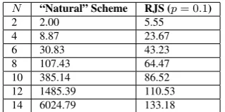
N “Natural” Scheme RJS (p= 0.1)
2 2.00 5.55
4 8.87 23.67
6 30.83 43.23
8 107.43 64.47
10 385.14 86.52
12 1485.39 110.53 14 6024.79 133.18
Table 2 Simulated average hitting time for the RJS scheme and the “natural” scheme for varyingN
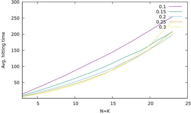
In Figure 3 we consider for different fixed values ofpthe hitting times for the worst-case type(N)for varyingN =K. We have considered values ofpfrom 0.1 to 0.9 with a spacing of 0.05, but we only show curves forpup to0.3, as larger values of
plead to very large hitting times for increasingN. These averages have been obtained by simulation, each point is the average of 20,000 replications. The figure suggests that:
– The average hitting time grows quickly inNfor fixedp.
– AsN grows, the value ofpthat gives the smallest hitting time becomes smaller, e.g. forN ≤10the best value ofpis 0.4, for11≤N ≤14the best value is 0.3 and so forth. We hypothesize that the optimal jumping probability forN, K→ ∞
while keepingK≤Nwill approach zero asymptotically.
In Table 1 we provide forN = K = 175, starting type (175)andp = 0.1 some summary statistics of one particular simulation run, where we record for each step in the simulation the number of balls in the most occupied bin and count how often a certain maximum bin occupation has occured. It can be seen that≈99.4%out of a total of 17,331 steps taken have a maximum occupation of either 2 balls (≈84%) or 3 balls (≈15.4%). This suggests that for larger values ofN the influence of the type of the starting state (here: the worst-case type(K)) is negligible and most of the time is spent in states with several bins having two or three balls only.
[image:13.595.161.321.197.277.2]N =Kand taken over 1,000,000 replications are shown in Table 2. It is evident that the “natural” scheme shows very poor performance rather quickly.
3K ≤N: A One-Bit Extension
The RJS algorithm discussed so far has desirable design properties (it does not require any coordination and converges with probability one to a non-colliding state when
K ≤ N) but the hitting time performance for larger values ofN andKappears to have room for improvement. We present an algorithm which retains those desirable properties and achieves much better hitting times, at the expense of three additional configuration parameters, which are probability values, and one additional bit of state besides the (dynamically changing) jumping probabilitypin each node. We refer to this algorithm as RJS-OB (where OB stands for “one bit”).
The basic idea of the proposed RJS-OB algorithm is that a ball which has “owned” a bin for at least one time slot (by which we mean that during this slot the ball was the sole occupant of this bin) is much more reluctant to leave this bin upon the next collision than another ball which has jumped into this bin. The RJS-OB scheme works as follows:
– Each nodeicarries one additional bit, denoted asoi (for “ownership”) and ini-tialized to 0 orFALSE. The jumping probabilitypifor this node is initialized to some valueq∈(0,1).
– At the beginning of a time slot nodeigoes through two distinct steps:
– In the first step it evolves its jumping probabilitypi: if the current bin is non-colliding (i.e. nodeiis the sole occupant), it setsoito 1 (or TRUE) and its jumping probability topi=qO, whereqO∈[0,1]is a parameter (the “owner probability”). If the bin is colliding andoi= 1(i.e. the node is the “owner”), it updates its jumping probability aspi := min{pi+qI, qN}, whereqIandqN are again fixed parameters (“probability increment” and “non-owner probabil-ity”). Otherwise, if the bin is colliding andoi = 0, thenpiis set topi=qN.
– In the second step the node, if colliding, uses its newly updated jumping prob-abilitypito make a random decision on whether to jump to another bin. If so, each of the otherN−1bins is chosen with equal probability and the flagoiis set to 0 (orFALSE). The jump is executed shortly before the end of the time slot.
By setting the “ownership probability” qO to a small value (e.g. qO = 0.05), the increment probabilityqI to a small value (e.g.qI = 0.01) and the non-ownership probabilityqN to a relatively large value (e.g.qN = 0.99) we achieve a behaviour where a node that owns a slot jumps with only small probability (but growing after repeated collisions), whereas another node which just jumped into the same bin will jump again with high probability. We assess the impact of some of these parameters on the hitting time below.
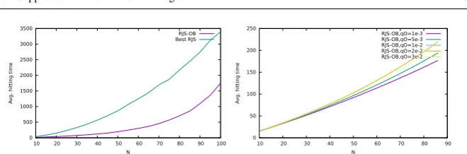
0 500 1000 1500 2000 2500 3000 3500
10 20 30 40 50 60 70 80 90 100
A
vg. hitting time
N
RJS-OB Best RJS
(a) RJS-OB withqO = 0.05,qI= 0.01,qN=
0.99and the best RJS(p) scheme for various val-ues ofp
0 50 100 150 200 250
10 20 30 40 50 60 70 80 90
A
vg. hitting time
N
RJS-OB,qO=1e-3 RJS-OB,qO=5e-3 RJS-OB,qO=1e-2 RJS-OB,qO=2e-2 RJS-OB,qO=3e-2
(b) RJS-OB with varying values of owner proba-bilityqO(withqI= 0.01andqN= 0.99)
Fig. 4 Average hitting times for RJS-OB scheme
In Figure 4(a) we show the results for an experiment in which we have variedN
and have assumed thatK = N holds. Furthermore, the system starts in the worst-case starting state of type(K). We show the average hitting time (obtained over 5,000 replications, where in each replication we run rounds until a non-colliding state has been reached) for the RJS-OB scheme (withqO= 0.05,qI = 0.01,qN = 0.99) and compare this against the best possible hitting time achievable with the RJS scheme after trying, for eachN, various values of the jumping probabilityp(we have varied
pfrom 0.01 to 0.4 in steps of 0.01). Clearly, the RJS-OB scheme is a significant improvement over the stateless RJS, which we attribute to the reluctance of balls “owning” a slot to jump away quickly after occasional collisions.
In Figure 4(b) we assess the impact of one particular parameter, the owner proba-bilityqOwhile keepingqI = 0.01andqN = 0.99fixed. The hitting times have been obtained over 1,000,000 replications. It can be seen that smaller values of the owner probability (i.e. a stronger reluctance of a settled ball to leave its bin) lead to reduc-tions of the hitting time and seem to approach a “linear” behaviour. We will return to this in Section 4.
4K ≤N: The Sticky Variant
We have observed for the RJS-OB scheme described in Section 3 that forK≤Nthe average hitting time appears to approach a linear behaviour for smaller and smaller values of the ownership probabilityqOasNandKincrease (see Figure 4(b)). In this section we analyse a particular variant of the RJS-OB algorithm in whichqO = 0,
qI = 0andqN = 1, i.e. balls owning their slot never move away and non-owning colliding balls always jump away. We refer to this as thesticky variant, as owners stick to their bin. In this section we design and evaluate a Markov model of the sticky variant which, by making an inconsequential extra assumption, is vastly simplified as compared to the model set up for the RJS scheme and has a much smaller state space size.
[image:15.595.77.407.74.183.2]including the slot it currently resides in – this assumption removes the necessity to keep track of the particular bin in which a colliding non-owner ball resides.3 Note
that forK > N the sticky variant will be very unfair in the long-term, asN of the balls will eventually own a slot and the remainingK−Nballs will never settle. We will assumeK≤N throughout this section.
0 50 100 150 200 250
0 20 40 60 80 100 120 140
A
vg. hitting time
N
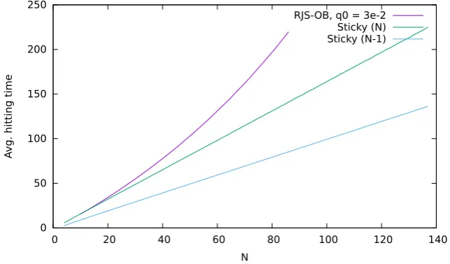
RJS-OB, q0 = 3e-2 Sticky (N) Sticky (N-1)
Fig. 5 Average hitting times for the RJS-OB scheme with owner probabilityqO= 3e−2and the sticky
scheme withK=Nballs andK=N−1balls
In Figure 5 we compare the average hitting times of the best RJS-OB scheme from Figure 4(b) against the sticky scheme for varyingN = K(all the times have been obtained by simulation). We have also added results for the sticky scheme with
K=N−1balls. It can be seen that indeed the sticky scheme shows an almost lin-ear scaling behaviour (it is not perfectly linlin-ear though), and furthermore that leaving away only one ball already provides substantial performance benefits. In the remain-der of this section we develop a Markov chain model for the sticky variant, analyze some of its properties, and present a mixture of analytical and numeric results related to the asymptotic growth of the average hitting time for increasingNandK.
4.1 Markov Model for the Sticky Variant
Since a colliding ball can jump into any bin, there is no need to keep track of the bin in which a colliding ball currently resides. Therefore, it suffices to use the number of owning or “settled” balls as state variable – recall that a ball is settled in a bin 3 We have furthermore confirmed through simulations (not reported here for space reasons) that already
[image:16.595.78.400.175.364.2]when it was the sole occupant for at least one time slot (after which it claims owner-ship). The state space isS={0,1, . . . , K}, and we denote the(K+ 1)×(K+ 1) state transition matrix byP. Since the number of settled balls never decreases,P= [[pi,j]]i,j∈{0,1,...,K} is an upper-triangular matrix with pK,K = 1, i.e. the state in which all balls are settled is absorbing. All other states are transient and have a non-zero probability to jump into the absorbing state, which guarantees that the absorbing state will be reached with probability one. The starting state is normally the state 0, i.e. the state in which there are not yet any settled balls. Note that the diagonal entries
pS,S(forS∈ S) are the eigenvalues ofP.
The transition probabilities are derived in Appendix B using the framework of exponential generating functions. The probability to go from stateSto stateS+T
forT ≥0is given by:
pS,S+T = N−S
T
·(K−S)!·PK−(S+T)
ν=0 (−1)
ν N−(S+T) ν
(N−T−ν)K−(S+T)−ν (K−(S+T)−ν)!
NK−S
(8) which forT = 0simplifies to:
pS,S =
(K−S)!·PK−S
ν=0 (−1) ν N−S
ν
(N−ν)K−S−ν (K−S−ν)!
NK−S (9)
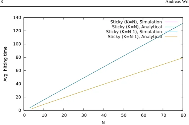
We have validated the analytical model for the state transition matrixPagainst empirical transition matrices obtained from Monte-Carlo simulations.4 In Figure 6
we compare the average hitting time for the simulation model (where the average is taken over 1,000,000 replications for givenN andK) and the analytical model. In both cases we start with 0 settled balls. It can be seen that they are in excellent agree-ment, as the curves for the simulation and analytical models overlap. However, the explicit forms of the transition probabilities (Equations (8) and (9)) are not particu-larly convenient.
4.2 Properties of the Transition Matrix
We here collect a few properties of the state transition probability matrixP= [[pij]]i,j∈S for the sticky variant. First, the diagonal entriesλS :=pS,Sare positive and strictly monotonically increasing inS, and we havepK−1,K−1= KN−1 andpK,K= 1. This is verified in Appendices C and D. Hence, the upper-triagonal transition matrixP hasK+ 1distinct eigenvalues and is diagonalizable. Secondly, forK ≥ 3all en-tries above the diagonal are strictly positive, except for entry[[P]]0,K−1= 0. This is verified in Appendix D.
4 The calculations for the analytical model of the transition matrixPhave been carried out with
Mathematicac and are exact. The empirical transition matrix for given values ofNandKhas been
esti-mated by simulating, for each start states0from 0 toK−1, a number of one million one-step transitions
and counting how often each possible successor state is assumed. From these counts we can calculate the transition probabilities. We have repeated this forN=Kranging fromN=K= 10toN=K= 150
0 20 40 60 80 100 120 140
0 10 20 30 40 50 60 70 80
A
vg. hitting time
N
Sticky (K=N), Simulation Sticky (K=N), Analytical Sticky (K=N-1), Simulation Sticky (K=N-1), Analytical
Fig. 6 Average hitting times for the Sticky variant, comparing simulation and analytical model (assuming
K=Nballs).
Thirdly, from any start statej∈ {0, . . . , K−1}the speed of convergence to the single absorbing stateK is at least geometric with rateλn
K−1 = K−1
N
n
, where
λK−1 =pK−1,K−1 = KN−1 is the second-largest eigenvalue ofP. In other words, afterntransitions the difference between one and the probability to be in the absorb-ing stateKis bounded byλnK−1times a constant independent ofn. This is shown in Appendix E.
4.3 Asymptotics for Average Hitting Time
We conclude the investigation of the sticky variant by considering what happens for
N, K → ∞(while K ≤ N) and provide a simple bound as well as conjectures suggested by (limited) numerical evidence. In all of the following we assume that we start in state 0.
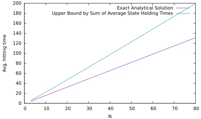
Given that from a stateS ∈ S we can never move into a smaller stateS0 < S, a coarse upper boundUN,K on the average hitting time is given by the sum of all average state holding times:
UN,K= K−1
X
S=0 1 1−pS,S
(10)
where the average state holding time 1−p1
[image:18.595.75.401.69.284.2]upper bound against the exact analytical solution for the average hitting time.5It can
be seen that the upper bound is not tight, but shows an almost linear behaviour.
0 20 40 60 80 100 120 140 160 180 200
0 10 20 30 40 50 60 70 80
A
vg. hitting time
N
Exact Analytical Solution Upper Bound by Sum of Average State Holding Times
Fig. 7 Average hitting times for the Sticky variant, comparing analytical model and upper bound given by sum of state holding times (assumingK=Nballs).
We have conducted extensive numerical experiments (using exact calculations) to conjecture better upper bounds. Our starting point is Equation (29) for starting state
j= 0. When we introduce the shorthand
CN,K,n
=−
λ
0
λK−1
n
u0,0v0,K+. . .+
λ
K−1
λK−1
n
u0,K−1vK−1,K
we get that
E[M0] = ∞
X
n=0
λnK−1·CN,K,n
The numerical experiments suggest that:
– When for givenN we consider all the possible values forK≤Nthen
CK,N,n≤
N
3 resulting in
E[M0]≤
N2
3(N−K+ 1) (11)
5 Both values have been obtained with Mathematicac using exact calculations. The analytical solution
[image:19.595.77.399.137.327.2]– For the case where we keep the difference betweenNandKfixed toC=N−K
we seem to have
CK,N,n≤C+ 2 resulting in
E[M0]≤
N(C+ 2)
C+ 1 (12)
These conjectures have been numerically confirmed for allN ≤50. For larger values ofN the computation time required by the exact calculations (which involve factors of the size ofN!) quickly becomes prohibitive.
5K > N: The One-Bit Extension in Overload Situations
The design of the RJS-OB scheme, and particularly the sticky variant, is geared to-wards reducing the average hitting time for the case K ≤ N, i.e. with at most as many balls as there are bins. Clearly, this condition cannot be guaranteed in real ap-plications and hence it becomes important to study the performance of the RJS-OB scheme in the scenarioK > N as well, where the hitting time is not meaningful anymore. For this study we use two main performance measures:
– Theaverage percentage of successful slots, defined as follows: for a particular ball we measure the percentage of all rounds in which the ball is the sole occupant of a slot and can successfully use it for data transmission. The average is then taken over all the balls.
– By its construction and depending on its parameters, the RJS-OB scheme intro-duces differences between balls by making some “owners” of a bin and others not (particularly when the owner probabilityqOand the probability incrementqI are configured to small values). It becomes possible that the owners receive a higher percentage of successful slots than the non-owners. To measure this unfairness we use thecoefficient of variation of the percentage of successful slots(or simply coefficient of variation). In general, the coefficient of variation (CoV) of a posi-tive random variable is defined as its standard deviation divided by the mean, and is a measure of variability. In our particular setting we measure the coefficient of variation of the percentage of successful slots of the different balls. Larger values of the CoV indicate larger differences within the node population.
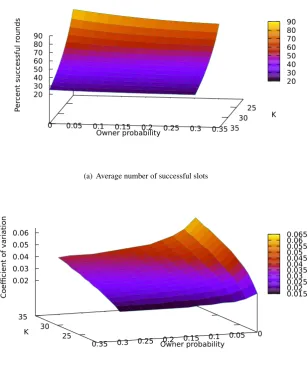
We have instrumented our simulation model to measure these quantities. For all re-sults we have used 10,000 rounds within a single simulation run, and for each set of parameters (we have variedN,K,pOandpN) we have carried out 10,000 dent replications, and in the following we report averages taken over these indepen-dent replications.
In the first set of results shown in Figures 8(a) and 8(b) we report both perfor-mance measures in a scenario where we have varied bothN andKin a manner that
0 5 10 15 20 25 30 0 0.05 0.1 0.15 0.2 0.25 0 10 20 30 40 50 60 70 80 90 Per
cent successful r
ounds
K
Probability Owner
Per
cent successful r
ounds 0 10 20 30 40 50 60 70 80 90
(a) Average number of successful slots
0 5 10 15 20 25 30 0 0.05 0.1 0.15 0.2 0.25 0.01 0.02 0.03 0.04 0.05 0.06 0.07 0.08 0.09 Coe ff of V
ariation Successful R
ounds K Probability Owner Coe ff of V
ariation Successful R
ounds 0.01 0.02 0.03 0.04 0.05 0.06 0.07 0.08 0.09
(b) Coefficient of variation
Fig. 8 Average number of successful slots and coefficient of variation for the RJS-OB scheme for varying
Kin an overload situation (N=K−2) and varyingqO
ratio K/N increases). Furthermore, the results shown in Figure 8(b) confirm that the owner probabilityqOhas significant impact on the coefficient of variation, with smaller values forqObeing more “unfair” than larger values.
[image:21.595.83.408.107.511.2]25 30 35
K 0 0.05 0.1 0.15 0.2 0.25 0.3 0.35
Owner probability 20
30 40 50 60 70 80 90
Per
cent successful r
ounds
20 30 40 50 60 70 80 90
(a) Average number of successful slots
25 30 35
K 0.1 0.05 0
0.15 0.2 0.25 0.3
0.35 Owner probability
0.02 0.03 0.04 0.05 0.06
Coe
ffi
cient of variation
0.015 0.02 0.025 0.03 0.035 0.04 0.045 0.05 0.055 0.06 0.065
(b) Coefficient of variation
Fig. 9 Average number of successful slots and coefficient of variation for the RJS-OB scheme forN= 20
and varyingKandqO(each point is furthermore averaged over different values forqN).
[image:22.595.94.403.116.484.2]substantially. Similarly, as the owner probabilityqOincreases, the percentage of suc-cessful slots decreases as well, although more moderately. Similarly, both parameters influence the coefficient of variation: increasingKincreases the CoV, and decreasing the owner probabilityqO increases the CoV as well, again highlighting the stronger unfairness when slot owners are too unwilling to give their slot up.
0 5 10 15 20 25 30 35 40 45
0 0.05 0.1 0.15 0.2 0.25 0.3 Owner probability
[image:23.595.87.398.175.366.2]Simulation results Asymptotic limit for pure balls-in-bins
Fig. 10 Percentage of successful slots forN = 20,K = 30,qN = 0.25and varyingqO, comparing
between RJS-OB and asymptotic value for static balls-in-bins allocation.
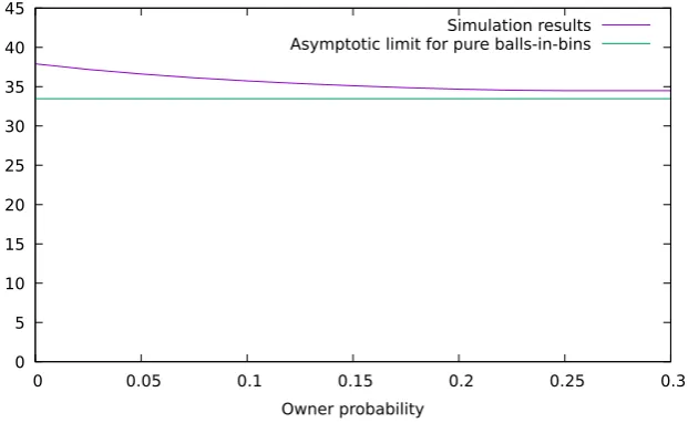
Finally, to show another perspective, in Figure 10 we show simulation results for the percentage of successful slots for the RJS-OB scheme with the non-owner proba-bility fixed toqN = 0.25,Nfixed toN = 20,Kfixed toK= 30, and varying owner probabilityqO. We compare the RJS-OB scheme against the theoretical asymptotic average percentage of bins with exactly one ball when using a pure balls-in-bins al-location. This asymptotic estimate is known to equaleKN ·K
N, see [14, p. 177]. These results suggest that by being unfair, the RJS-OB scheme can achieve somewhat better percentages of successful slots than a pure balls-in-bins allocation, but with increas-ing owner probabilityqO(and thus increasing fairness) we approach from above the performance of pure balls-in-bins. This suggests an interesting item for future re-search, by providing balls (i.e. WBSNs) with the means to estimate the total number
K of balls in the system (we suppose thatN is usually known a-priori) and to its operational parametersqN andqOaccordingly.
6 Conclusions
of frequency channels. We argue that the RJS-OB scheme is the most promising, as it has shown good performance for the considered parameters (and certainly superior performance over the RJS scheme) and can settle into a non-colliding state easily (provided there exists one), it is not restricted to the caseK ≤N, and furthermore its behaviour can be adjusted for different population sizes.
There is significant potential for future work. For example, for the RJS-OB algo-rithm it would be interesting to develop good estimators for the numberKof WBSNs present in the system (assuming thatN is known a-priori) and to track this number when the population changes over time, e.g. due to WBSNs leaving or joining ei-ther as individuals or in batches. Next, assuming thatK andN are known, it will be important to identify good values for the parametersqO,qN andqI, so that in the caseK ≤ N the average hitting time is minimized, whereas in the caseK > N
we want to allocate undisturbed transmission opportunities in a fair manner. It will also be interesting to transfer the algorithm to a scenario without central slotted time, where each node makes decisions asynchronously (see for example [4]), or to situa-tions where a frequency can host a variable number of WBSNs subject to a constraint that the total load does not exceed a threshold.
With respect to the sticky variant, it would be very interesting to confirm or refute the asymptotic results for the average hitting time of the sticky scheme (Equations (11) and (11)) which express the seemingly linear behaviour for fixed difference be-tweenN andK. Another interesting question is whether the RJS-OB or the sticky scheme can be improved upon by introducing more than one bit of additional state.
A Reducing System Size in Equation(5)
In this appendix we discuss how to reduce the size of the linear equation system (5) and (6), making it more accessible to numerical solution. The key roles are played by the notion of types introduced in Section 2 and the exploitation of symmetries.
To begin with, it is straightforward to see that we only need to consider terms for the colliding states in Equation (6), as the hitting times in non-colliding states are always zero. Next, consider two colliding statessaandsbof the same type. Therefore, there exists a permutationσ(·)of the bins from1toN
such thatsb = σ(sa). From the definition of the transition probabilities (Equations (3) and (4)) it is
straightforward to check thatp(t|s) =p(τ(t)|τ(s))holds for any permutationτ(·), and therefore the vector(p(t|sb) :t∈ CN,K)of transition probabilities from statesbto all colliding states is a permutation
of the vector(p(t|sa) :t∈ CN,K), as applying the permutationσ(·)to all colliding states reproduces
the entire set of colliding states.
Next, fix two different typesT(s)andT(t). Since all states of the same typeT(s)are permutations of each other, a similar argument shows that the vector of transition probabilities(p(t0|sa) :t0∈ T(t))
from some statesa∈ T(s)to all states inT(t)is a permutation of the transition probabilities(p(t0|sb) :t0∈ T(t))
from any other statesb ∈ T(s)to all states inT(t). If we now order the states according to their type
(i.e. all states of the same type are grouped together) and leave out the non-colliding states, then the matrix of state transition probabilities for the remaining states can be written as a block matrix of the following form:
P0=
A((KK)) A((KK−)1,1) . . .A((2K,1),...,1)
A((KK−)1,1) A((KK−−11,,1)1) . . .A(2(K,1−,...,1,1)1)
. . . .
A((2K,1),...,1)A((2K,1−,...,1,1)1). . .A(2(2,,11,...,,...,1)1)
where the matrixAT1
T2contains all transition probabilities from statess∈ T1to statest∈ T2, and in such
from (6) can be re-arranged as
P0−I
·k= (−1,−1, . . . ,−1)T (13)
wherekis the solution vector with the hitting times of all non-colliding states andIis the identity matrix of suitable dimension. Please note that in this equation the matrix(P0−I)maintains the property of matrix
P0of being a block matrix made up of matrices where all the rows are permutations of each other: in all
the “diagonal matrices”AT
T the respective diagonal elements are identical and remain so after subtracting
the identity matrix. Furthermore, since we have omitted all transitions into non-colliding states (which occur with positive probability from every colliding state), the matrixP0is strictly sub-stochastic, which in turn makes the matrix(P0−I)strictly diagonal-dominant and thus the equation system (13) is uniquely solvable. Note that its dimension is given by the size of the state space|SN,K|with only the non-colliding
states removed.
The key property which now allows to simplify the calculation of the hitting times is that all states of the same type have the same average hitting time. To see this, we argue as follows. If we denote byαT1
T2
the row sum of sub-matrixAT1
T2, then the system
α((KK)) α((KK−)1,1) . . . α((2K,1),...,1)
α((KK−)1,1) α((KK−−11,,1)1) . . . α(2(K,1−,...,1,1)1)
. . . .
α((2K,1),...,1)α((2K,1−,...,1,1)1). . . α(2(2,,11,...,,...,1)1)
−I
·k0= (−1,−1, . . . ,−1)T (14)
is again strictly diagonal-dominant and thus has a unique solutionk0= (k(K), k(K−1,1), . . . , k(2,1,...,1)).
Furthermore, its dimension is given by the number of typesCKexisting forKballs (minus one, the
non-colliding type(1,1, . . . ,1)– compare Equation (7)). We construct a vectorkfromk0by starting with
repeating valuek(K)exactly|T(K)|times, followed by|T(K−1,1)|repetitions ofk(K−1,1)and so
forth. It is then clear that this vectorkis a solution of the full equation system (13).
Let us consider the savings that can be obtained from using system (14) instead of (13). ForN= 15
andK= 10we have thatC10= 42and thus the system (14) has to be solved for 41 unknowns (after
leaving out the single non-colliding type). As discussed before in Section 2.2, the full system (13) would have a dimension in the order of approximately 1.9 million unknowns.
B Sticky Variant: Derivation of Transition Probabilities
To derive explicit expressions for the transition probabilities of the sticky model we will use the framework of exponential generating functions (EGF) [14], [38], [27]. When applying EGF to balls-in-bin problems, a modified exponential power series
c(z) =
∞
X
m=0
cm
m!z
m (z∈
C) (15)
is associated to each bin, where the coefficientscm ∈ {0,1}are chosen to express whether or not it
is permissible to havemballs in the bin. The power series for several bins are then multiplied to get the overall EGF for the problem, and them-th coefficient of the overall EGF gives the total number of allocations of balls to bins which satisfy all constraints simultaneously.
Exponential generating functions are one widely used class of generating functions, another class are ordinary generating functions. EGFs are appropriate in settings with labeled (i.e. distinct) entities. When given a general power seriesf(z), we denote by{zn}f(z)the coefficient for theznterm off(z), and
for the particular case of an EGFc(z)formed according to Equation (15), the coefficientcmis given by cm=m!· {zm}c(z). Note that an EGFc(z)(taken as a power series aroundz = 0) is an analytic /
holomorphic function within its convergence radius, and it is a basic fact from complex analysis that we can recover the coefficients of a power seriesc(z)from the derivatives ofc(z):
cm
m!=
(∂mc)(0)
where∂mdenotes them-th complex derivative operator.
To transition from stateS∈ S to stateS+T ∈ S we find the number of allocations ofK−S
unsettled balls to bins such that
– Each of theSbins containing a settled ball can contain zero or more unsettled balls. To each such bin we assign the EGFez, in which all coefficients are one (compare Equation (15)).
– T of the bins that contained no settled ball before should now contain exactly one ball. To each of these bins we assign the EGFz(corresponding toc1= 1andcm= 0form6= 1).
– The remainingN−S−T bins each contain either zero or at least two balls. To each of these bins we assign the EGF(ez−z), excluding the case of exactly one ball.
The EGF corresponding to these constraints is given by
f(z) = (ez)S·zT·(ez−z)N−(S+T) (17)
and the expression(K−S)!·
zK−S f(z)gives the number of such allocations. This expression,
however, refers to one particular choice ofTbins out of theN−Sbins not containing a settled ball, and there are in total NT−Ssuch choices. Therefore, the total number allocations ofK−Sunsettled balls to bins satisfying the above constraints is given by
n(S, T) =
N−S
T
·(K−S)!·nzK−S
o
f(z)
(18)
and since the total number of allocations ofK−Sballs toN bins is given byNK−Sthe transition
probability becomes
pS,S+T=
n(S, T)
NK−S =
N−S T
·(K−S)!·
zK−S f(z)
NK−S (19)
To get explicit expressions, we expand the term(ez−z)N−(S+T)of Equation (17) using the binomial
theorem, and simplify the resulting expression (exploitingK≤N) to arrive at:
n(S, T) =
N−S
T
·(K−S)!· (20)
K−(S+T) X
ν=0
(−1)νN−(S+T)
ν
(N−T−ν)K−(S+T)−ν
(K−(S+T)−ν)!
which forT = 0simplifies to
n(S,0) = (K−S)!·
K−S
X
ν=0
(−1)νN−S ν
(N−ν)K−S−ν
(K−S−ν)! !
(21)
Note that a straightforward calculation yields that in particular we have
pK,K = 1 (22)
pK−1,K−1 =
K−1
N (23)
pK−2,K−2 =
N+K2−5K+ 6
N2 (24)
C Sticky Variant: Monotonicity of Self-Transition Probabilities
In this Appendix we show that the self-transition probabilitiespS,Sin the Markov model of the sticky
vari-ant (compare Equations (20) and in particular (9)) are strictly monotonically increasing inSforK≥2, i.e. that forS∈ {0,1, . . . , K−1}we havepS,S< pS+1,S+1. Note that the self-transition
jump with positive probability back to exactly where they currently are, so that they remain in the colliding state.
The EGF corresponding to the diagonal entries can be specialized from Equation (17) for fixed state
Sto become:
fS(z) =ezS·(ez−z)N−S (25)
by settingT = 0, and valid for all0 ≤S ≤K ≤N. When taken as a power series, note thatfS(z)
has non-negative coefficients, sinceg1(z) =ez = 1 + z
1!+
z2
2! + +
z3
3! +. . .andg2(z) =e
z−z=
1 +z2!2+z3!3+. . .have only non-negative coefficients andfS(z)is formed out ofg1(z)andg2(z)by
multiplications. Note that the power seriesg3(z) =zalso has only non-negative coefficients.
We can say more: forS6= 0a factorg1(z)is present which has strictly positive coefficients through-out, and all other factors offS(·)contribute a 1, so infS(·)there is at least one term of any order and
all the coefficients are truly positive. ForS= 0all coefficients offS(·)of order zero or of order two or
more are strictly positive. The coefficient of order one (for the termz) is zero, but this is relevant only for
K= 1. So for allK≥2and allSthe coefficients offS(·)are strictly positive.
From the general expression for the transition probabilities (Equation (8)) and by taking into account that extracting coefficients is equivalent to taking derivatives (Equation (16)) we get
pS,S=
(K−S)!·
zK−S f
S(z)
NK−S
=
(K−S)!·h∂K−SfS(0)
(K−S)!
i
NK−S
= ∂K−SfS(0)
NK−S (26)
With this, the conditionpS,S< pS+1,S+1is equivalent to the condition
∂K−S
h
ezS(ez−z)N−S i
(0)
< N·h∂K−S−1 h
ez(S+1)(ez−z)N−S−1i(0)i (27)
ForS= 0the left-hand side of this relation becomes
∂K−1 h
∂1(ez−z)N i
(0) =N·∂K−1 h
(ez−z)N−1·(ez−1) i
(0)
and the right-hand side will be
N·h∂K−1 h
ez(ez−z)N−1 i
(0) i
Plugging this back into condition (27) after cancelingN, subtracting the left-hand side from the right-hand-side and using the linearity of the derivative we get the condition
0< ∂K−S
h
ez(ez−z)N−1−(ez−z)N−1·(ez−1)i(0)
=∂K−S
h
(ez−z)N−1(ez−(ez−1)i(0)
=∂K−S
h
(ez−z)N−1i(0)
which is just extracting theK−Scoefficient out of a power series (an integer power ofg2(z)) with coefficients that are non-negative in general and strictly positive from thez2coefficient onwards. Hence,
forN ≥ K≥2andS= 0the claim is true. For0 < S ≤K−1we get for the left-hand side of condition (27):
∂K−S−1 h
∂1 h
ezS(ez−z)N−Sii(0)
=∂K−S−1 h
With this the condition to check becomes
0< ∂K−S−1 h
N ez(S+1)(ez−z)N−S−1−SezS(ez−z)N−S−ezS(N−S) (ez−z)N−S−1(ez−1) i
(0)
=∂K−S−1 h
ezS(ez−z)N−S−1(N ez−S(ez−z)−(N−S) (ez−1))i(0)
=∂K−S−1 h
ezS(ez−z)N−S−1(Sz+ (N−S))
i (0)
which again is built from (a sum of) products ofg1(z),g2(z)andg3(z)and has strictly positive coeffi-cients, verifying the claim.
D Sticky Variant: Strict Positivity of Transition Probabilities
In this Appendix we argue that the transition probabilities above the diagonalpS,S+T(withT >0) in
the Markov model of the sticky variant (compare Equations (20) and in particular (9)) are strictly positive, with one exception.
The starting point is again the EGFf(z)from Equation (17), which is a product of integer multiples of the three elementary EGFsg1(z) =ez,g2(z) =ez−zandg3(z) =z.
The case of a state0< S < Kis straightforward: the EGFf(z)contains the factorzTand the two other factors(g1(z))Sand(g2(z))N−(S+T)both contribute az0= 1term, so thezTterm inf(z)is
strictly positive.
For the stateS= 0we distinguish three cases:
– WithT =Kwe are asking about state transition probabilityp0,Kwhich from elementary
combina-torial considerations is given byN·(N−1)·. . .·(N−K+ 1)>0.
– WithT =K−1we are asking that we are jumping out of a state in which no ball is settled into a state where every ball but one is settled – but to make this happen the firstN−1balls must jump alone into an empty bin (otherwise they would not settle) and the remaining ball cannot jump into the same bin as any of the others (otherwise none of the two would settle), so the last ball must jump into another empty bin, where it settles. More formally, forS= 0andT =K−1we get the generating functionf(z) =zK−1·(ez−z)N−K+1which forK ≥3does not contain a term inz, so the
coefficient forz(and thus the transition probability into this state) are 0.
– For1≤T ≤K−2the argument is very similar to the argument forS >0.
E Sticky Variant: Convergence Speed towards Absorbing State
The claim of a geometric convergence speed of the Markov chain for the sticky variant towards the absorb-ing state 0 is in itself not a surprise, as it is similar to well-known results from the literature (compare for example [5, Chap. 6]), but the proofs of these frequently rely on the Perron-Frobenius theorem, which is only valid for irreducible transition matrices, which our upper-triagonal matrixPwith the entries derived in Appendix B is not. We therefore proceed to verify this directly. SincePis diagonalizable (compare Section 4.2), we can expressPasP=U·D·U−1=:U·D·V, whereD= diag(λ
0, λ1, . . . , λK)
is a diagonal matrix made up of the eigenvalues / diagonal elements ofPand the columns ofUare given by the (linearly independent) right eigenvectorsxifor eigenvaluesλi.
LetMjbe a non-negative, integer-valued random variable denoting the number of steps it takes to
get from starting statej ∈ {0, . . . , K−1}to the absorbing stateK. The average hitting time is then the expectationE[Mj]. For this expectation we can use the well-known so-called survivor representation
[27]:
E[Mj] =
∞
X
n=0
Pr [Mj> n]
If we denote by[v]ithei-th component of a vectorvthen we clearly have from the setup of our system that
holds, whereekis thek-th unit vector inRK+1(taken as a row vector here). RecallingλK= 1we get
[ej·Pn]K
= [ej·U·Dn·V]K
=λn0uj,0v0,K+λn1uj,1v1,K. . .+λnK−1uj,K−1vK−1,K+uj,KvK,K
Since convergence to the absorbing state happens with probability one and recallingλi < 1fori ∈
{0,1, . . . , K−1}we see
0 = lim
n→∞[eK−ej·P n]
K
= 1−uj,KvK,K (28)
and therefore
[eK−ej·Pn]K (29)
=− λn0uj,0v0,K+λn1uj,1v1,K. . .+λnK−1uj,K−1vK−1,K
=−λnK−1
λ0
λK−1
n
uj,0v0,K+. . .+
λK−1
λK−1
n
uj,K−1vK−1,K
≤λnK−1· kujk2· kvk2
(using the abbreviationsuj = (uj,0, uj,1, . . . , uj,K−1)andv= (v0,K, v1,K, . . . , vK−1,K)). This
verifies the claim.
References
1. Ahmed, E., Gani, A., Abolfazli, S., Yao, L.J., Khan, S.U.: Channel Assignment Algorithms in Cogni-tive Radio Networks: Taxonomy, Open Issues, and Challenges. IEEE Communications Surveys and Tutorials18(1) (2016)
2. Baker, S.B., Xiang, W., Atkinson, I.: Internet of Things for Smart Healthcare: Technologies, Chal-lenges, and Opportunities. IEEE Access5, 26,521 – 26,544 (2017)
3. Berenbrink, P., Brinkmann, A., Friedetzky, T., Meister, D., Nagel, L.: Distributing Storage in Cloud Environments. In: Proc. IEEE 27th International Symposium on Parallel and Distributed Processing, Workshops and PhD Forum (IPDPSW). Cambridge, Massachusetts, USA (2013)
4. Berenbrink, P., Kling, P., Law, C., Mehrabian, A.: Tight Load Balancing via Randomized Local Search. In: Proc. IEEE 27th International Symposium on Parallel and Distributed Processing (IPDPS). Orlando, Florida, USA (2017)
5. Bremaud, P.: Markov Chains – Gibbs Fields, Monte Carlo Simulation, and Queues. Springer, New York (1998)
6. Cavallari, R., Martelli, F., Rosini, R., Buratti, C., Verdone, R.: A Survey on Wireless Body Area Networks: Technologies and Design Challenges. IEEE Communications Surveys and Tutorials16(3) (2014). Http://www.comsoc.org/livepubs/surveys
7. Chieochan, S., Hossain, E., Diamond, J.: Channel assignment schemes for infrastructure-based 802.11 WLANs: A survey. IEEE Communications Surveys and Tutorials12(1) (2010)
8. Choi, J.S., Zhou, M.: Performance analysis of zigbee-based body sensor networks. In: Systems Man and Cybernetics (SMC), 2010 IEEE International Conference on, pp. 2427–2433. IEEE (2010) 9. Degesys, J., Rose, I., Patel, A., Nagpal, R.: DESYNC: Self-Organizing Desynchronization and TDMA
on Wireless Sensor Networks. In: Proc. Symposium on Information Processing in Sensor Networks (IPSN ’07). Cambridge, Massachusetts, USA (2007)
10. Deligiannis, N., Mota, J.F.C., Smart, G., Andreopoulos, Y.: Fast Desynchronization for Decentralized Multichannel Medium Access Control. IEEE Trans. Communications63(9), 3336–3349 (2015) 11. Demir, L., Kumar, A., Cunche, M., Lauradoux, C.: The Pitfalls of Hashing for Privacy. IEEE
13. Fischer, S., Maehoenen, P., Schoengens, M., Voecking, B.: Load Balancing for Dynamic Spectrum Assignment with Local Information for Secondary Users. In: Proc. 3rd IEEE Symposium on New Frontiers in Dynamic Spectrum Access Networks (DySPAN). IEEE, Chicago, Illinois, USA (2008) 14. Flajolet, P., Sedgewick, R.: Analytic Combinatorics. Cambridge University Press, Cambridge, UK
(2009)
15. Goodman, D.J., Valenzuela, R.A., Gayliard, K.T., Ramamurthi, B.: Packet reservation multiple access for local wireless communications. IEEE Trans. Communications37(8), 885–890 (1989)
16. Johnson, N.L., Kotz, S.: Urn Models and their Applications. John Wiley & Sons, New York (1977) 17. Kenney, J.B.: Dedicated Short-Range Communications (DSRC) Standards in the United States.
Pro-ceedings of the IEEE99(7), 1162–1182 (2011)
18. Kolchin, V.F., Sevast’yanov, B.A., Chistyakow, V.P.: Random Allocations. Vh Winston (1978) 19. LAN/MAN Standards Committee of the IEEE Computer Society: IEEE Standard for Local and
metropolitan area networks – Part 15.6: Wireless Body Area Networks (2012)
20. LAN/MAN Standards Committee of the IEEE Computer Society: IEEE Standard for Low-Rate Wire-less Networks – IEEE Std 802.15.4-2015 (2015)
21. Latre, B., Braem, B., Moerman, I., Blondia, C., Demeester, P.: A survey on wireless body area net-works. Wireless Networks17, 1–18 (2011)
22. Levin, D.A., Peres, Y., Wilmer, E.L.: Markov Chains and Mixing Times. Americal Mathematical Society, Providence, Rhode Island (2009)
23. Li, Q., Yang, P., Tang, S., Xiang, C., Li, F.: Many is Better than All: Efficient Selfish Load Balancing in Mobile Crowdsourcing Systems. In: Proc. Third International Conference on Advanced Cloud and Big Data. Yangzhou China (2015)
24. Liggett, T.M.: Interacting Particle Systems. Springer, Berlin (2008)
25. Liu, T.K., Silvester, J.A., Polydoros, A.: Performance evaluation of R-ALOHA in distributed packet radio networks with hard real-time communications. In: Proc. 45th IEEE Vehicular Technology Con-ference (VTC), pp. 554–558 (1995)
26. Moravejosharieh, A., Willig, A.: Mutual Interference in Large Populations of Co-Located IEEE 802.15.4 Body Sensor Networks – A Sensitivity Analysis. Elsevier Computer Communications81, 86 – 96 (2016)
27. Nelson, R.: Probability, Stochastic Processes, and Queueing Theory – The Mathematics of Computer Performance Modeling. Springer Verlag, New York (1995)
28. Neugebauer, M., Pl¨onnigs, J., Kabitzsch, K.: A new beacon order adaptation algorithm for ieee 802.15. 4 networks. In: Wireless Sensor Networks, 2005. Proceeedings of the Second European Workshop on, pp. 302–311. IEEE (2005)
29. Norris, J.R.: Markov Chains. Cambridge University Press, Cambridge, UK (1997)
30. Park, Y., Kim, H.: Collision Control of Periodic Safety Messages With Strict Messaging Frequency Requirements. IEEE Trans. Vehicular Technology62(2), 843 – 852 (2013)
31. Petrova, M., Olano, N., Maehoenen, P.: Balls and Bins Distributed Load Balancing Algorithm for Channel Allocation. In: Proc. 7th IEEE/IFIP International Conference on Wireless On-demand Net-work Systems and Services (WONS), pp. 25 –30. Kranjska Gora, Slovenia (2010)
32. Qiang, L., Jun, T.: Minimum-energy-cost algorithm based on superframe adaptation control. In: Com-munications (ICC), 2011 IEEE International Conference on, pp. 1–5 (2011)
33. Sari, R., et al.: Analysis of the effect of beacon order and superframe order value to the performance of multihop wireless networks on ieee 802.15. 4 protocol. In: Advanced Computer Science and Information Systems (ICACSIS), 2012 International Conference on, pp. 89–94. IEEE (2012) 34. Seneviratne, S., Hu, Y., Nguyen, T., Lan, G., Khalifa, S., Thilakarathna, K., Hassan, M., Seneviratne,
A.: A Survey of Wearable Devices and Challenges. IEEE Communications Surveys and Tutorials
19(4) (2017). Http://www.comsoc.org/livepubs/surveys
35. Siavoshani, M.J., Pourmiri, A., Shariatpanahi, S.P.: Storage, Communication, and Load Balancing Trade-off in Distributed Cache Networks. IEEE Trans. Parallel and Distributed Systems29(4), 943 – 957 (2018)
36. Tao, Z., Panwar, S., Gu, D., Zhang, J.: Performance analysis and a proposed improvement for the ieee 802.15.4 contention access period. In: Wireless Communications and Networking Conference, 2006. WCNC 2006. IEEE, vol. 4, pp. 1811–1818. IEEE (2006)
37. Wei Zhang and Timothy Wood and Jinho Hwang: NetKV: Scalable, Self-Managing, Load Balancing as a Network Function. In: Proc. IEEE International Conference on Autonomic Computing (ICAC). Wuerzburg, Germany (2016)