Development of a multi-rotor platform
with integrated thrust sensors
J.L.J. (Jasper) Scholten
MSc Report
Committee:
Prof.dr.ir. S. Stramigioli
Dr.ir. T.J.A. de Vries
Dr.ir. M. Fumagalli
Prof.dr.ir. G.J.M. Krijnen
October 2014
Development of a multi-rotor platform with integrated thrust sensors
Jasper L.J. Scholten
Abstract— The work presented in this paper focuses on the design and realization of a micro sized multi-rotor Unmanned Aerial Vehicle (UAV) with integrated thrust sensors. The goal has been to use the measured (actual) thrust in a feedback loop for thrust control for each motor and propeller, during flight. Furthermore, the aim has been to create a low-cost and easy to use multi-rotor research platform. The multi-rotor consists of a single printed circuit board, weighs approximately 99 grams (without battery) and measures 226 [mm] x 226 [mm] with propellers. Strain gauges positioned on the arms that connect the actuators to the base of the multi-rotor are used to measure the thrust. The UAV features a 10 degree of freedom Inertial Measurement Unit (IMU) and optionally the Gumstix Overo computer-on-module (RAMstix software compatible), together with its camera, the Caspa FS/VL. Because of its modular design, the multi-rotor can be extended by user designed modules and supports several communication modules with varying ranges (indoor [<100m], outdoor [>1km]), connection speeds (250kbps-2Mbps) and several standards (Bluetooth, WiFi). Proper functioning of the realized UAV has been shown by means of submodule tests. Further testing is needed, in which the usefulness of the thrust sensor should be demonstrated. One problem was surfaced though; the arms exhibit an unwanted torsional vibration that results in unreliable electrical connec-tions.
I. INTRODUCTION
In the last decade there has been an increasing interest in aerial robotics; especially in multi-rotor platforms, because of their simplicity of construction, their ability to hover and their ability to vertically takeoff and land (VTOL). The last few years, it has been possible to create smaller micro aerial robots with better performance and more advanced features. These small micro aerial robots have received great attention due to the favorable scaling laws; e.g. with respect to their agility [1] and due to their potential fields of application, such as swarm formations.
In [2], [1] and [3], micro-sized multi-rotors are presented that represent the current state-of-the-art. In [2], an 86g, 232 mm diameter open source micro UAV is created that is constructed on a single Printed Circuit Board (PCB). It has a 9 Degree of Freedom (DoF) Inertial Meaurement Unit (IMU) and a Gumstix Overo [ref:gumstix] compute-on-module that is able to run the Robot Operating System (ROS). In [1], a 73g, 210 mm diameter micro quad-rotor is presented that is able, due to its agility, to operate in a team of 20 micro quad-rotors in swarm formations. In [3], a 128g, 260 mm diameter quad-rotor is developed with an on-board FPGA for image processing, giving it the possibility to perform visual feature detection of the ground and as a result, operate autonomously.
The dynamics of multi-rotors have been researched pro-foundly in the last decade; e.g. [4], [5]. To control the
motors of a multi-rotor, often a static relationship between the actuator’s speed and the thrust generated is assumed [4]. Given the desired thrust, the required angular velocity of the rotor is computed, which is then used by a speed controller to control the rotor’s speed. This scheme however has problems in dealing with aerodynamic effects, such as the ground effect [6] or wind disturbances that are either not rejected by the control law [7] or require a sophisticated control law [8], [9], [10].
In [11], an adaptive Luenberger observer is used to es-timate the thrust of each individual actuator. A hardware-in-the-loop simulation, consisting of a 1 degree of freedom system, has been preformed to validate the presented ob-server. However, it is based on a linear model that neglects nonlinear cross coupling terms and therefore only applicable to near hover operations.
[image:2.612.326.545.464.584.2]In [12], estimates of both the rotor’s speed and motor current are used to estimate and control the aerodynamic power. Although regulating aerodynamic power is not the same as controlling the actual thrust, the algorithm is shown to be more robust against aerodynamic effects such as axial and horizontal airflow disturbances. As a result, it outper-forms current state-of-the-art motor controllers that control the rotor’s angular velocity, but hasn’t been implemented and tested on a flying UAV.
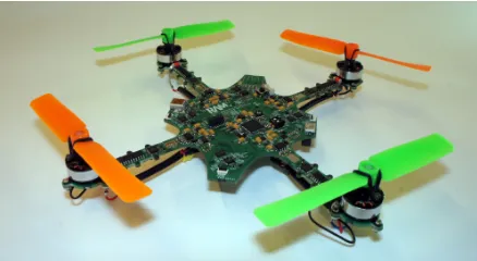
Fig. 1. Designed multi-rotor with integrated thrust sensors.
This paper proposes a novel scheme where, instead of a model based thrust estimation approach, an attempt is made to control the actual thrust of each actuator by use of integrated thrust sensors. In this first step, a new micro UAV multi-rotor has been designed (Figure 1) to incorporate thrust sensors while also providing an new agile research platform. The UAV is made out of a single printed circuit board that simplifies its design and fabrication. Furthermore, it facilitates the integration of thrust sensors.
This paper is organized as follows: in Section II, the
elty is analysed and the performance determining parameters are identified. In Section III, the design of the multi-rotor is presented, after which in Section IV the control scheme is discussed. In Section V, the experiments performed and the results obtained are presented. Finally in Section VI a conclusion is drawn and recommendations are made.
II. ANALYSIS
In order to measure the thrust, the idea is to integrate thrust sensors, in the form of strain gauges, in the arms of the multi-rotor as illustrated in Fig. 3. The thrust generated by each actuator creates a moment of force at each point located on the arm. Once a specific point is chosen, due to bending, a strain occurs which can be measured and interpreted as a stress depending on the mechanical properties of the arm. Under the assumption that a homogeneous linear elastic material is used in its stress range, Hooke’s law is valid and the strain is proportional to the stress at the point of interest. It is this strain that can be measured by means of strain gauges (as the name suggests). As a result, implementing strain gauges on the arms of a multi-rotor enables the measurement of the thrust forces:
= L·d
I·E·FT (refer to Fig. 2) (1)
x y z F L M
d
TFig. 2. Illustration of strain measurement whereMis the moment of force created by the forceFT and armL.
where is the strain, FT the thrust, L the length of the arm,dthe distance between the location of the strain gauge and the arm’s neutral axis,I the area moment of inertia and E the Young’s modulus of the material.
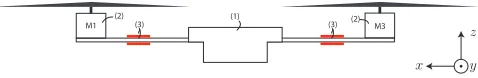
[image:3.612.315.560.102.216.2](1) (2) (2) (3) (3) x y z M1 M3
Fig. 3. Cross section of a multi-rotor. With (1), the integrated electronics and battery, (2) the motors and their corresponding propellers, (3) the integrated strain gauges used to measure the thrust.
However, a multi-rotor is best viewed as a floating me-chanical system; in other words, it has no connection with the fixed world. Due to the fact that several sources of force are present, the strain measured by each strain gauge is not only due to the corresponding actuator’s thrust. To further analyse this, a simple model, represented by the iconic diagram in Fig. 4, is created. This model is analysed in Section II-A.
In Section II-B it is determined whether thrust control can be achieved and in Section II-B.3 insight is gained in the performance limitations. dis F base m m cb F b c m cb F b c T
F (t) (t) FT(t)
(t) (t)
Case Case Case
TS TS
x y
z
b
[image:3.612.77.297.335.455.2](m ,J b)
Fig. 4. A 1D model of a multi-rotor’s cross section. Case{1,2,3}represent the cases that will be analysed whileT Srepresent the Thrust Sensor.
The following notation is used throughout this analysis: HB
A denotes the transfer function fromAtoB,FT xdenotes the (thrust) force of actuator x and Fcby denotes the force
between the base of the multi-rotor and actuator y. Fur-thermore, most equations are linear and written in Laplace domain and therefore, where possible,(s)is omitted.
The following coordinate definition is used (refer to Fig. 5): the x-axis of the multi-rotor is aligned with actuator 1 and 3 and points from the center of the PCB towards motor 1, while the y-axis is aligned with actuator 2 and 4 and points to motor 2. τx denotes the torque about the x-axis and is created by actuator 2 and 4.τy denotes the torque about the y-axis and is created by actuator 1 and 3. τz is the torque about the z-axis and is created by all four actuators. The rotation direction of the first and third motor are opposite to the rotation direction of the second and fourth motor and hence always have a negative magnitude. Thereforeτ1 and τ3 are likewise negative in magnitude and as a result,tzcan be controlled in both directions.
x y z F2 F1 F3 F4 m2 m3 m1 B m4 ω3 ω2 ω1 ω4
Fig. 5. Illustration of the multi-rotor’s body fixed frame, thrust and angular velocities.
A. Model analysis
[image:3.612.316.558.493.656.2] [image:3.612.59.298.565.604.2]mass of the base of the multi-rotor is represented bymbase and this mass includes its inertia. Furthermore, the following assumptions are applicable:
1) The actuators and base of the multi-rotor are rigid. 2) The operating regime of the arms is such that Hooke’s
Law is valid at all times.
3) Each thrust sensor (T S), i.e. arm with strain gauge, is modeled as an ideal force sensor, measuringFcby(t), in
series with an ideal spring. The corresponding spring constant beingcby. The spring represents the (bending) stiffness of the arm in the operating area defined in item 2. In general the damping does not dominate the dynamics of the mechanism and will only complicate the considerations that follow. Therefore, the damping is neglected.
4) The forces acting on the multi-rotor are the thrust forces FT x on the actuators and a disturbances force Fdis(t)on the base of the multi-rotor. The forces include all aerodynamic effects and hence represents the total aerodynamic force.
The following three cases are now analysed:
1) One actuator without disturbance force (cb3is decoupled andFdis remains zero).
2) One actuator with disturbance force (cb3is decoupled). 3) Two(+) actuators with disturbance force.
Case 1) One actuator without disturbance force: In [13], classes of electromechanical motion systems are introduced for fourth-order mechanisms. The system in this first case, a mass-spring-mass plant of the fourth-order, corresponds to a flexible mechanism. Once the location of the actuator and sensor are chosen, the plant’s transfer function can be derived. The denominator polynomial of the plant’s transfer function is independent on the location of the actuator and sensor. The numerator polynomial however does depend on the location of the actuator and sensor.
In motion control applications, as considered in [13] the goal is to control the displacement or velocity of the end-effector. Therefore, the focus lies on the open loop transfer function from the actuator’s forceFT1(t)to the displacement or velocity of the mass whose position or velocity is mea-sured. However, in this case the goal is to control the thrust force and hence, the focus lies on the open loop transfer function from the actuator’s forceFT1(t)to the force exerted on the base of the multi-rotor (Fcb1).
Due to the location of actuator FT1 and sensor Fcb1, the following open-loop transfer function is derived:
Fcb1 =H cb1
FT1·FT1 (2)
with:
Hcb1 FT1 =
cb1 m1
s2+cb1 m1
+cb1 mb
= ω
2
ar,m1 s2+ω2
r
(3)
ωr= s
cb1 mbase
+cb1 m1
(4)
ωar,m1 = s
cb1 m1
(5)
Equation 3 can be characterised as a standard second order low pass transfer function with two poles (±ωri) located on the imaginary axis in the pole-zero map. These poles determine the bandwidth of the system (eq. 4) and introduce a total phase shift of −π. Even though no anti-resonance frequency is present, cb1
m1 does represents a time constant in the numerator and therefore is represented by ωar,m1. For low frequencies equation 3 converges to:
Hcb1 FT1(0) =
ω2
ar,m1 ω2
r
(6)
The maximum achievable gain is unity and therefore the highest measurement sensitivity within the bandwidth of the system is achieved when:
|Fcb1(jω)|=|FT1(jω)| ∀ω∈[0, ωBW) (7)
The bandwidth of the system (ωBW) in case no damping is present is defined asωr.
Case 2) One actuator with a disturbance force: In this second case a disturbance force is added to the system. By use of the superposition principle, the force measured by the force sensor can be described by equations 3, 8, 9 and 10.
Fcb1 =H cb1
FT1·FT1−H cb1
dis·Fdis (8)
Hcb1 dis =
cb1 mb
s2+ cb1 m1
+cb1 mb
= ω
2
ar,mb
s2+ω2
r
(9)
ωar,mb=
s cb1 mb
(10)
As mentioned, the only difference between the open loop transfer functions,Hcb1
dis andH cb1
FT1, is the numerator:ω 2
ar,m1 versusω2
ar,mb. The denominator of the plant’s transfer
func-tion and therefore, the bandwidth and resonance frequency remain the same. As a result, only the steady state gain of both open loop transfer functions differ. For most multi-rotors, the mass of the actuator is smaller than the mass of its base, and thus the disturbance force is attenuated with a higher degree than the thrust force:
|Hcb1
dis(jω)|<|H cb1
FT1(jω)| ∀ω (11)
Case 3) Two(+) actuators with disturbance force: In this last case a second actuator is added to the system. The open loop transfer function is still rather simple to express, especially when taken into account the system has a symmetry:
Hcb1 dis =H
cb3 dis =H
c
dis (12)
Hcb1 FT1=H
cb3 FT3=H
c
FT (13)
yielding in terms of sensitivity:
Fcb{1,3}=SFT{1,3}·FT{1,3}−SFdis·Fdis−
SFT{3,1}·FT{3,1} (14)
SFT{1,3}=
Hc FT
1−(Hc dis)2
(15)
SFdis=
Hc dis−(H
c dis)
2
1−(Hc dis)2
(16)
SFT{3,1}=
Hc dis·H
dis c ·H
c FT
1−(Hc dis)2
(17)
Hdis
c = 1 (18)
For the complete derivation please refer to Appendix I. With respect to the second case, the second actuator increases the steady state gain of both sensitivity functions SFT{1,3} andSFdis. Furthermore a dependency on the thrust
force of the second actuator,FT3, is introduced.
From (3), (9) and (19) it can be deduced that for low frequencies, i.e.ωω{ar,r}, the following holds:
|SFT{1,3}(jω)|=|1−SFdis(jω)|
=|1−SFT{3,1}(jω)| (19)
Symbolic analysis has shown that the measured force for a multi-rotor with four actuators equals:
Fcby =S
y
FT y·FT y−S
y
dis·(Fdis+ X
i6=y
FT i) (20)
For a multi-rotor with four actuators equation 19 remains valid and is not influenced by mass variations of the actuators and stiffness variations of the multi-rotor’s arms. However, variations do result in the introduction of more resonance and anti-resonance frequencies. As a rule of thumb, the lowest (anti-)resonance frequency can be approximated by the combination of arm and actuator that lead to the lowest (anti-)resonance frequency. For the complete derivation refer to Appendix I-B.
B. Thrust control
In order to evaluate whether thrust control can be achieved, it has to be determined what the inputs of a multi-rotor are and how these are being controlled. For a multi-rotor with four actuators four degrees of freedom can be controlled namely, three rotational DoFs and one translational DoF: the (vertical) translation in its z-axis. In order to control these
four DoFs the actuator’s thrust force has to be mapped to the total thrust force and torque about each axis (refer to Fig: 5): Fz τx τy τz =
1 1 1 1
0 darm 0 −darm
darm 0 −darm 0
−k k −k k
·
Fcb1 Fcb2 Fcb3 Fcb4
(21)
Heredarm denotes the distance between the actuator and the multi-rotor origins.kdenotes the thrust to torque coeffi-cient of the actuator and is often empirically determined. These desired thrust forces are now in general converted by a static relationship to an angular velocity. This angular velocity is then used to control the speed of the actuator in a closed loop.
In case a feedback loop around the measured force is formed, a mapping is required from the thrust force and torques to the measured forceFcby. As the measured forces
do not only depend on FT y it has to be determined if and how the thrust force and torques can be mapped to the measured forces. Furthermore, if a mapping exists, it has to be determined what the limitations are and how these can be influenced.
At first, for both the thrust force and torques it is deter-mined if they can be mapped, after which the limitations are determined.
1) Thrust force: In section II-A it has been shown that the measured forces depend on both the disturbance force and all thrust forces. The translational dynamics of a multi-rotor with four actuators, expressed in its body fixed frame, can be expressed as:
mbase·v˙ b,0
b =
4
X
y=1
Fcby+Fdis (22)
Here vbb,0 represents the velocity of the multi-rotor’s base (b) with respect to the inertial frame of reference (0) and expressed in the multi-rotor’s body fixed frame (b).
In the absence of a disturbance force, by controllingFcby
the total thrust force can be controlled. In case a disturbance force is present and the measured force is regulated, any error in the state of the multi-rotor is caused by the disturbance force. Moreover, as the measured force depends on the disturbance force, a part of the disturbance force is rejected by closing the loop around the measured forceFcby.
2) Torques: In order to determine the torques about the x and y-axis of the multi-rotor, knowledge of the actual actuators their forces (FT x) and the distances between the actuators and the multi-rotor’s origin are required. In this case, a measurement is available (Fcby) in which FT y is
tried:
τx=darm·(FT2−FT4), try: τx=darm·(Fcb2−Fcb4)
Using equation (20) this yields:
τx=darm·
(S1
FT1+S 3
dis)·FT1−
(S3
FT3+S 1
dis)·FT3−
(S1
dis−S
3
dis) X
i=2,4,dis FT i
(23)
In case the arms and actuators are well matched, i.e. equa-tions 12 and 13 are valid, S1
dis becomes equal to Sdis3 and thus the disturbance forces cancel out. Furthermore S1
FT3 becomes equal to S3
FT3 and as a result, the following is deduced:
τm{x,y}= ω2
r,mact
s2+ω2
r,mact
·τ{x,y} (24)
ωr,mact=
s c mact
(25)
and for the torque about the z-axis:
τmz= ω2
r,mact
s2+ω2
r,mact
·τz (26)
In other words, in case equations 12 and 13 are valid, all torques acting on the multi-rotor can be measured within the bandwidth of the system. As a result the desired torques can be mapped to the measured forcesFcby.
3) Limitations: More insight in the proposed scheme is required to determine its limitation as in reality the actuators will vary in mass as does the stiffness of the arms. By introduction of the following mass ratio, the limitations can be expressed more clearly.
Rm= mbase
mact
(27)
withmact being the average mass of the actuators.
The influences of mass variations of the actuators can be determined by defining the mass of the actuators as follows:
m{1,2,3,4}=mact·(1 +X{1,2,3,4}) (28)
where X{1,2,3,4} is the deviation of each actuator with respect to the average actuator’s mass.
Now the measured thrust force for a multi-rotor with four actuators can be expressed for low frequencies, i.e. ω
ω{ar,r}, as (refer to equation 20 and Appendix I-B):
Fcbx(0) =
3 +Rm+Pi6=xXi
4 +Rm+P4i=1Xi
·FT x(0)−
X
i6=x
1 +Xx 4 +Rm
·FT i(0)− 1 +Xx 4 +Rm
·Fdis(0) (29)
Fcbx(0) =
3 +Rm 4 +Rm
·FT x(0)−
X
i6=x 1 4 +Rm
·FT i(0)− 1 4 +Rm
·Fdis(0) (30)
As the stiffness constants are not present in equation (30) stiffness variations of the multi-rotor’s arm do not influence the measured force. Variations in the actuator’s mass do influ-ence the measurement, but do not impact the performance of a closed loop thrust controller as the loop is closed around the measured force. The achievable bandwidth is determined by the anti-resonance and resonance frequencies present. These frequencies should be obtained from numerical analysis or simulation but, in case the mass and stiffness of each arm and actuator is well matched, i.e. no mass/stiffness variations, Hcby
FT y equals:
Hcby
FT y =
ωr,my
s2+ω
r,my
·3·c+Rm·c+Rm·m·s 2
4·c+Rm·c+Rm·m·s2 (31)
Hence the lowest resonance frequencies is ωr,my. In case
of mass or stiffness variations, as a rule of thumb, the lowest frequency can be approximated by the combination of actuator’s mass and stiffness that lead to the lowest frequency.
With the introduction of the mass ratio and the definition of the actuator’s mass, the error in the torque measurement for low frequencies, i.e. ω ω{ar,r}, can be expressed as (refer to equation 23 and Appendix I-B):
τe{x,y}(0) = (1−
4 +Rm+X2+X4
4 +Rm+P
4
i=1Xi
)·τ{x,y}(0)+
( 2·X{3,4} 4 +Rm+P
4
i=1Xi
)·FT{1,2}(0)−
( 2·X{1,2} 4 +Rm+P4i=1Xi
)·FT{3,4}(0)−
X
i={2,1},{4,3},dis
( X{3,4}−X{1,2} 4 +Rm+P
4
i=1Xi
)·Fi (32)
It can be concluded that a variation of the actuator mass of 10% together with a mass ratio of 10 creates an uncertainty of 2.9 % plus an additional torque error of1.45%·|τ{x,y}(0)|. Furthermore 1.45% of the disturbance force and the other actuator’s thrust forces are measured. These errors will result in inaccuracy of the torque to force mapping.
In order to reduce this error an high mass ratio is required. In case the mass ratio converges to infinity the measured
force converges to:
lim
Rm→∞Fcby =
ωr,my
s2+ω
r,my
·FT y (33)
And hence the torque converges to:
lim
Rm→∞τm{x,y}=
ωr,m{2,1}
s2+ω
r,m{2,1}
·FT{2,1}− (34)
ωr,m{4,3}
s2+ω
r,m{4,3}
·FT{4,3} (35)
The dependency on the disturbance force has been elim-inated and for low frequencies, i.e. ω ωar,r, the error converges to zero.
Finally, it can be concluded that for torque measurement a high mass ratio is desired while for the thrust force a trade-off is formed. This is, because for the thrust force measurement to be insensitive to the disturbance force an high mass ratio is required. This enables, in case the state of multi-rotor is known, to determine the disturbance force. On the other hand, a low mass ratio enables better control of the total thrust force as a larger part of the disturbance force is reflected in the measurements and therefore can be rejected. As for the torque measurements, a low mass ratio increases the error in the mapping significantly and therefore an high mass ratio is required. Furthermore, the measured torque, in case the desired accuracy can be met, can be used to improve the attitude estimation and hereby further improve the performance; again stressing the importance of an high mass ratio.
III. MULTI-ROTORDESIGN
r =51 5
124
124
Gumstix
motor c ontrol
thrust sensor
IMU
[image:7.612.79.275.446.647.2]SG
Fig. 6. Design of the multi-rotor with integrated thrust sensors. For one arm the position of the motor controller and thrust sensor is drawn. The Gumstix Overo, outlined with dash lines, is located at the bottom side of the multi-rotor. 5 [mm] of spacing is used between the propeller and the base of the multi-rotor to minimize the disturbance of the airflow.
In [14], a preliminary multi-rotor design has been made which is based on user requirements [15] and experimental
results of the available combinations of micro-sized motors and propellers. Given these results, the designed multi-rotor uses 4” inch (101.6 mm) propellers. Together with the main user requirements of an optional Gumstix with camera(s) and preferable high mass ratio, this has led to the design of the multi-rotor’s main board as shown in Fig. 6.
In total, the multi-rotor electronics consist of two 6-layers printed circuit boards; the main board and a power supply board. The main board forms the frame of the multi-rotor and houses all the electronics except the power supply electronics; these are located on the power supply board. This power supply board distributes power to the subsystems, including the actuators, and is to be attached to the bottom of the main board.
The overall dimensions of the multi-rotor are 226 [mm] by 226 [mm] and it weighs 99 grams. This is without battery and additional modules attached. The mass ratio, as introduced in the analysis, depends on the battery used and with either an 1800mAh 11.1V battery or an 950mAh 11.1V battery, the mass ratio equals 5.1 respectively 3.7. The corresponding hover time equals (theoretically) 26 minutes respectively 20 minutes and a thrust to mass ratio of 2.3 respectively 3.3 is obtained.
For a mass ratio of 5.1 a mass variation of 10% will now, in theory, result in an error in the torque measurement of 4.5% plus a maximum of 2.25 % of the actual torque and disturbance force is measured. This holds for frequencies lower than the lowest resonance frequency present. The lowest resonance frequency, formed by the stiffness of the arm and mass of the actuator, is approximated to be equal to 50 Hz. This frequency can however, in case experiments deem this necessary, be increased by adding external support to stiffen the arm section holding the motor controller and motor. This support can be mounted to the six mounting holes that are located on the arms as shown in Fig. 6.
The thrust sensors, in the form of (semiconductor) strain gauges, are located on pads on both the top and bottom side of the arms (SG in 6). As they are placed in a half-bridge configuration, the measurement is insensitive to changes in the temperature. Furthermore, as they are placed in the center of the arm’s longest axis, i.e. aligned with the multi-rotor’s x and y axis, axial strain is rejected.
For future research projects it is possible to add additional modules via the corresponding mounting holes and electronic headers, including USB peripherals. This gives the user the option to attach modules like a GPS module, cameras, ultrasound altitude sensors etcetera.
In the next section a systematic overview of the system is presented and its main parts are discussed shortly.
A. System overview
In Fig. 7 a systematic overview of the multi-rotor is shown with all its subcomponents and connections.
Low Level Controller SPI RF module header SPI USB Analog/Digital I/O header Gumstick UART USB Loop Controller Motor controller Gumstick camera IMU 10DoF SPI I/O header 3 axis Accelerometer 3 axis Magnetometer 3 axis Gyroscope Barometer Strain gauge's ADC 1 2 3 5 SPI SPI type A/B type A/B type A USB type A/B
WiFi/Bluetooth
[image:8.612.54.298.54.211.2]4
Fig. 7. Designed multi-rotor with integrated thrust sensors.
with the loop controllers that control the motor controllers. Each main subcomponent, numbered in Fig. 7, is discussed below.
1) LLC: the low lever controller is a 8/16-bit RISC based microcontroller running at 32 MHz (AtXmega128A3U). It has, among other features, multiple SPI interfaces, an event and Direct Memory Access (DMA) controller and a full-speed USB interface. Each peripheral that requires direct communication with the LLC has been assigned a dedicated SPI interface. Furthermore all SPI interfaces can make use of the event and DMA controller; this increases the communication speed by offloading the CPU. The event system furthermore facilitates real-time performance, which can be crucial during complex flight maneuvers. The USB interface can be used, together with a boot-loader, to program the microcontroller and for debugging purposes. The choice for the XmegaAVR series has been made because users familiar with either the AVR series from Atmel or with an Atmel based Arduino should find the switch to the XmegaAVR series rather painless compared to switching to an ARM-based microcontroller.
2) a) LC: the loop controller is a 8-bit RISC based micro-controller running at 16MHz (Atmega88PA). Its main task is to control the speed of the motor. The speed reference is received from the LLC and the actual speed from the motor controller (MC). Its output is a Pulse Width Modulation (PWM) duty cycle which is sent to the motor controller via its second SPI interface. Its second task is to acquire the Analog Digital Converter’s (ADC) result of the strain gauge measurement and eventually control the (thrust) force in a feedback loop.
b) MC: the motor controller is also an 8-bit RISC based microcontroller running at 16MHz, but from the tinyAVR series (ATtiny861). It features an on board PLL oscillator that is able to create a fast peripheral clock of 64MHz. This clock is used to create three 10 bits PWM signal with a modulation frequency of 20kHz. These PWM signals are used to control the
motors. The main task of the motor controller is to start the motor and keep the motor running with the desired PWM duty cycle. Due to the control being sensorless, this task uses most of the CPU’s time, which is why the LC has been introduced.
3) The multi-rotor currently houses two sensor devices, one barometer and one 9-axis motion sensor, which together form the 10 Degree of Freedom Inertial Mea-surement Unit of the multi-rotor. The 9-axis motion sensor (MPU9250) includes an 3-axis accelerometer, a 3-axis gyroscope and a 3-axis magnetometer all in one single package. The accelerometer and magnetometer enable the determination of the absolute attitude while the gyroscope enables the determination of faster mo-tions. Via a single SPI interface (or I2C) the data of all three internal sensors can be acquired. The barome-ter (MS5607-02BA03), accessible via SPI, enables the multi-rotor’s altitude to be determined with a resolution of 20[cm].
4) For communication with the user, an RF module can be attached to the multi-rotor. Currently, a 2.4GHz module (nRF24L01+) is used which supports communication speeds up to 2 Mbps with an indoor range of roughly 30 meters. Due to the modular design, other com-munication modules (e.g. nRF905) that utilize lower frequencies (e.g. [433/868/915MHz]) can be used to extend the range, at the cost of data throughput. 5) For use with more sophisticated control algorithms or
Digital Signal Processing (DSP), a Gumstix Overo and its camera can be fitted to the multi-rotor. The mounting holes gives the user the ability to design custom brackets for Gumstix’s WiFi/Bluetooth antennas and camera(s).
IV. CONTROL
The introduction of a closed loop thrust controller in-creases the number of cascaded controllers. As a result, the control structure of a UAV consist of three cascaded control loops as is shown in Figure 8. Note that often, an additional position loop is present and thus four cascaded control loops are formed. In order for a cascaded controller to outperform a single controller, the loop rate of the inner controller has to be higher than the outer controller, preferably by a factor 10. In order to facilitate this control scheme, the following loop rates are implemented:
• Speed control: 10 kHz
• Thrust control: 2 kHz (not yet implemented, but sup-ported)
• Attitude control: 200 Hz
The loop rate should preferably be a factor 10 higher than the bandwidth of the system and therefore, a 20 Hz attitude bandwidth is possible. This bandwidth allows a multi-rotor to make acrobatic maneuvers in case the actuators have the required bandwidth. For the design multi-rotor a flip for example, in case a skew sine path is used with a PD
ω=f(FT ) Model inversion + -q* qm
C
q Motor dynamicsRotorω*
ω
Speed control
Attitude
Estimation τ=f(F )cbx
Thrust control
C
ωm
F cbx
C
FTM
+ -+ -Rigid body dynamics Attitude control [image:9.612.66.548.57.197.2]ω ,m-UAVa ,mmm
Fig. 8. Overview of the control structure of the multi-rotor.
controller, can be performed in 0.4 seconds with a tracking error of 2.9 degrees according to motion control theorems [13].
A. Attitude estimation and control
The attitude of the multi-rotor is currently estimated by use of the accelerometer, gyroscope and magnetometer. The data of these sensors is presented in the sensor’s body fixed frame and hence can be used to estimate the attitude of the multi-rotor in its body fixed frame. A complementary filter, which is less computational intensive than a conventional Kalman-based algorithm and has the same performance, is used to estimate the attitude in quaternion representation [16]. The advantage of the quaternion representation is that no singularities are present and only four values are required to represent that attitude of the multi-rotor [17].
Currently, after computation of the error quaternion, the simplest approach is taken to control the multi-rotor in near hover conditions. Although this approach is not singularity free, no singularities will be present as it is only being used for near hover conditions. This approach consist of mapping the error quaternion to yaw (z-axis), roll (x-axis) and pitch (y-axis) Euler angels. A PD controller is implemented on each axis to control the corresponding angles and henceCq (Fig. 8) consist of three PD controller. The PD controllers make use of the measured angular velocity of the gyroscopes (D-action) and the error angle (P-action). The gains have been tuned empirically.
V. EXPERIMENTAL VALIDATION
The following experiments have been performed: 1) Calibration of thrust sensor by using a sinusoidal speed
reference.
2) Research of the influence of the ground effect on the thrust measurements.
3) Research of the influence of a wall on the thrust measurements.
Furthermore all the subsystems of the multi-rotor have been successfully tested. The communication between the subsystems also work reliably. However, due to torsional
vibration of the arms, which are induced by the motors, several electrical connections on the arms have proved to be unreliable during take-off. As a result, the multi-rotor has yet to make its first flight and therefore only the mentioned experiments have been performed.
The setup for the performed experiments are discussed in Section V-A, after which the results are discussed in Section V-B. The results are evaluated in Section V-C.
A. Experimental setup
Fig. 9. Overview of the experimental setup
An overview of the test setup is given in Fig. 9. The experimental setup consist of the following modules:
1) The designed multi-rotor as described in Section III. The strain gauge’s signal is sampled at 2 kHz. A second order IIR filter is applied with a cut of frequency of 200 Hz.
2) F/T Sensor [18]: A six-axis force and torque sensor which is being used to calibrate and serve as reference for the thrust measurements. The sensor is mounted on a table and attached, via a bracket, to the multi-rotor’s base.
[image:9.612.334.532.372.515.2]being sent to the multi-rotor. After transmission of a acknowledged packet, the multi-rotor replies by sending a package. This package contains (desired) data that can be logged during the experiments. The ground station can also be interfaced with a joystick to generate the reference attitude. Both the measured attitude by the multi-rotor and the reference attitude can be displayed by use of Simulink’s 3D animation toolbox. This way, the quaternions can be represented in a simple and intuitive way.
B. Results
0 10 20 30 40 50 60
−2 0 2 4 time (s) Fo rc e (N)
0 10 20 30 40 50 60
0 1000 2000 3000 time (s) C om m ut at io n tim e (s
) Motor 3
[image:10.612.58.297.225.426.2]FT sensor Strain gauge
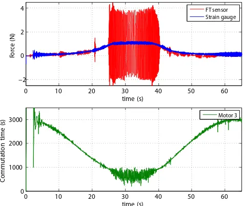
Fig. 10. Experiments 1: calibration measurement of the strain gauge located on the third arm. In the top plot the force measured by the strain gauge (blue) and the force measured by the F/T sensor (red) are shown. In the bottom plot the commutation time of the motor is shown which is inversely proportional to its speed.
In the top plot of Fig. 10 the force measured by the calibrated strain gauge and F/T sensor are shown. In the bottom plot the commutation time is shown. The commu-tation time is the time between two commucommu-tations of the brushless motor. This time is being measured by the speed controller and is inversely proportional to the speed of the motor; the speed of the motor is not measured directly. The motor controller might commutate to early or to late due to an incorrect detection of the motor’s orientation, especially at higher speed (refer to Fig. 10). As a result, and due to the relative slow dynamics of a motor, the commutation time consist of more high frequent signals, or peaks, than actual speed of the motor.
The calibration has been performed by both initializing the strain gauge measurement and F/T sensor force at zero. The gain has been determined by using the measured data from zero till 24 second. From 24 seconds till roughly 41 seconds the F/T sensor measures a large fluctuating force, which the strain gauge does not, or with a much lower amplitude, measure. Moreover, the vibrations cause an offset to occur in
the F/T sensor’s measurement, while no offset variations are present in the strain gauge’s measurement. An FFT analysis has shown that the fluctuating force lies in the frequency range of 10 to 18 Hz. Experiments in which the F/T sensor was being hold by hand, i.e. less rigidity and more vibrational damping than a table, resulted in a significant reduction of the fluctuation’s amplitude. Therefore, it is expected that the fluctuations in the F/T sensor’s measured force are due to the interconnection of the F/T sensor and the table.
During the first part of the measurement (5 till 8 seconds) and the last part (60 till the end), fluctuation of the measured strain gauge data can be observed. These however coincides with the speed of the actuator; an FFT analysis has shown that the fluctuation consist of an vibration with exactly the same frequency as the motor is running.
Because of the large fluctuations in the measurements of the F/T sensor, its results are left out in the sequel.
60 70 80 90 100 110 120 130
0 0.5 1 1.5 time (s) Fo rc e (N)
60 70 80 90 100 110 120 130
1000 1500 2000 time (s) C om m ut at io n tim e (u s) Fc b3 Fc b3 − Filtered ωm ω*
Fig. 11. Experiments 2: Influence of the ground effect on the force measured by the strain gauges. In the top plot the force measured by the strain gauge (blue) and its low pass filtered version are shown (red). In the bottom plot the measured commutation time of the motor (green) and the reference commutation time are shown (red).
In Fig. 11, the results of the second experiment are shown. During this experiment an large piece of paper is, at times, held below the multi-rotor’s propeller at a distance of 60 mm. This paper represents represents the situation where the multi-rotor has to fly over an object. At each vertical line in the figure the piece of paper is either added or removed.
The theoretically predicted ground effect is clearly re-flected in the measurements; adding a piece of paper results in a increase of average thrust increase of 7.8%, while removing it results in a (average) sudden thrust reduction of 12.4 %. This large reduction of thrust is expected to be due to the aerodynamics; the airflow requires time to recover. During each section the thrust is regulated with a standard deviation of 3.1 % of the average value. From 95 second onwards the commutation time has a standard deviation of 3.8% of its average value, although higher order frequent
[image:10.612.316.556.274.474.2]signals are present in this measure as mentioned.
160 165 170 175 180 185 190 195
0.7 0.8 0.9 1 1.1 time (s) Fo rc e (N)
160 165 170 175 180 185 190 195
600 800 1000 1200 time (s) C om m ut at io n tim e (u
s) ωm
[image:11.612.57.296.84.273.2]ω* Fc b3 Fc b3 − Filtered
Fig. 12. Experiments 3: Influence of an neighboring wall on the force measured by the strain gauges. In the top plot the force measured by the strain gauge (blue) and its low pass filtered version are shown (red). In the bottom plot the measured commutation time of the motor (green) and the reference commutation time are shown (red).
In Figure 12, the results of the third experiments are shown. During this experiment, which is performed after the second experiment, a large piece of paper representing a wall is folded around the propeller at a distance of 10mm, with the center of the paper aligned with the propeller axis. Adding the wall decreases the thrust with an average of 9.2 %.
C. Evaluation
All subsystem of the multi-rotor have proven to be op-erational and are able to successfully perform their tasks. However, torsional vibrations created unreliable electrical connections. As a result, the multi-rotor hasn’t made it first flight. These torsional vibration were detected during the design phase, but during that phase, the motors were not properly balanced which increased the induced vibrations. Furthermore, less induced vibration were expected during flight, as the multi-rotor becomes a floating mechanical system. Also, unreliable electrical connections were not detected.
The detection of the torsional vibration in the design phase has led to the design decision of making an option available to increase the torsional stiffness of the arms. This should lead to the attenuating of the induced vibrations. Moreover, not only can this option be used to stiffen the arms, it can also be used to reduce the stress on the components placed on the arms, thereby solving the unreliable electrical connections. In case, this does not solve the problem a redesign would be required. Components that are vulnerable to stress should in the redesign not be located on the arms.
From the first experiment it can be concluded that the setup in which the F/T sensor is mounted to a table is unsat-isfactory. The F/T sensor measures large force fluctuations which seem not be present in the strain gauge’s measurement.
However, they could be present with a smaller amplitude and therefore an new setup is required in which this problem is tackled. A setup in which the F/T sensor is suspended by ropes between two tables should eliminate this problem. The ropes, namely have a low bending stiffness while they still provide a high axial stiffness to keep the setup in place.
Nonetheless from all three experiment it can be concluded that the strain gauge is able to successfully measure the thrust. Furthermore the ground effect and the effect of flying close to a wall are clearly reflected in the thrust measurements. These effects result in a variation of the thrust that lies in the range of 7.8 % till 12.4 % of the its actual value. It is therefore expected that a thrust controller is able to attenuate this effect and hereby improve the multi-rotor’s performance.
VI. CONCLUSION
In this paper a new scheme is presented in which thrust sensors are used to control the thrust force of each individual actuator.
Analysis on the proposed scheme have been performed to determine its limitation. The analysis has shown that, not only the thrust force can be measured, but also the torques on the multi-rotor can be measured. These torque might be useful to improve the estimation of a multi-rotor’s state, but further research is required to determine its effectiveness. During the analysis a mass ratio has been introduced that determines the effectiveness of the proposed scheme. Ideally the mass ratio should be infinity which is difficult to achieve with conventional multi-rotor designs. New ways of designing a multi-rotor with as criteria the mass ratio should therefore be investigated profoundly.
A new multi-rotor platform has been presented that in-corporates thrust sensors. The multi-rotor platform does not only serve as platform to test the thrust sensors; the platform also serves as a new research platform. Its modular design gives the user the ability to add additional modules such as sensors or communication modules. Furthermore for image processing applications a Gumstix Overo, with an onboard DSP and additional cameras can be added to the multi-rotor. All the subsystem of the multi-rotor have successfully been tested and perform their tasks reliably. However, due to torsional vibrations, induced by the motors, electrical connections on the multi-rotor’s arm have proven to be unreliable. As a result, the multi-rotor has yet to make its first flight. This problem might however be easy to solve with the proposed modifications.
REFERENCES
[1] A. Kushleyev, D. Mellinger, C. Powers, and V. Kumar, “Towards a swarm of agile micro quadrotors,”Autonomous Robots, vol. 35, no. 4, pp. 287–300, 2013.
[2] C. Lehnert and P. Corke, “µav - design and implementation of an open source micro quadrotor,” inAustralasian Conference on Robotics
and Automation (ACRA2013)(J. Katupitiya, J. Guivant, and R. Eaton,
eds.), (University of New South Wales, Sydney, NSW), pp. 1–8, Australian Robotics & Automation Association, 2013.
[3] R. Konomura and K. Hori, “Designing hardware and software systems toward very compact and fully autonomous quadrotors,” inAdvanced Intelligent Mechatronics (AIM), 2013 IEEE/ASME International
Con-ference on, pp. 1367–1372, July 2013.
[4] S. Bouabdallah, P. Murrieri, and R. Siegwart, “Design and control of an indoor micro quadrotor,” in Robotics and Automation, 2004.
Proceedings. ICRA ’04. 2004 IEEE International Conference on,
vol. 5, pp. 4393–4398 Vol.5, April 2004.
[5] R. Mahony, V. Kumar, and P. Corke, “Multirotor aerial vehicles: Modeling, estimation, and control of quadrotor,”Robotics Automation
Magazine, IEEE, vol. 19, pp. 20–32, Sept 2012.
[6] C. Powers, D. Mellinger, A. Kushleyev, B. Kothmann, and V. Kumar, “Influence of aerodynamics and proximity effects in quadrotor flight,”
in Experimental Robotics (J. P. Desai, G. Dudek, O. Khatib, and
V. Kumar, eds.), vol. 88 of Springer Tracts in Advanced Robotics, pp. 289–302, Springer International Publishing, 2013.
[7] P. Martin and E. Salaun, “The true role of accelerometer feedback in quadrotor control,” in Robotics and Automation (ICRA), 2010 IEEE
International Conference on, pp. 1623–1629, May 2010.
[8] M. Orsag and S. Bogdan, “Hybrid control of quadrotor,” inControl
and Automation, 2009. MED ’09. 17th Mediterranean Conference on,
pp. 1239–1244, June 2009.
[9] H. Huang, G. Hoffmann, S. Waslander, and C. Tomlin, “Aerodynam-ics and control of autonomous quadrotor helicopters in aggressive maneuvering,” inRobotics and Automation, 2009. ICRA ’09. IEEE
International Conference on, pp. 3277–3282, May 2009.
[10] S. Lupashin, A. Schollig, M. Sherback, and R. D’Andrea, “A simple learning strategy for high-speed quadrocopter multi-flips,” inRobotics
and Automation (ICRA), 2010 IEEE International Conference on,
pp. 1642–1648, May 2010.
[11] A. Awan, J. Park, and H. J. Kim, “Thrust estimation of quadrotor uav using adaptive observer,” in Control, Automation and Systems
(ICCAS), 2011 11th International Conference on, pp. 131–136, Oct
2011.
[12] H. Bangura, M.and Lim, H. J. Kim, and R. Mahony, “Aerodynamic power control for multirotor aerial vehicles,” inRobotics and
Automa-tion, 2014. ICRA ’14. IEEE International Conference on, pp. –, May
2014.
[13] E. Coelingh, T. J. A. De Vries, and R. Koster, “Assessment of mecha-tronic system performance at an early design stage,” Mechatronics,
IEEE/ASME Transactions on, vol. 7, pp. 269–279, Sep 2002.
[14] J. L. Scholten, “Phase 1: experimental results and multi-rotor design decisions.” Attached as Appendix II.
[15] J. L. Scholten, “User Requirement Specifications (URS).” Attached as Appendix III.
[16] S. Madgwick, A. Harrison, and R. Vaidyanathan, “Estimation of imu and marg orientation using a gradient descent algorithm,” in
Reha-bilitation Robotics (ICORR), 2011 IEEE International Conference on,
pp. 1–7, June 2011.
[17] J. Chou, “Quaternion kinematic and dynamic differential equations,”
Robotics and Automation, IEEE Transactions on, vol. 8, pp. 53–64,
Feb 1992.
[18] ATI Net F/T Sensor System. http://www.ati-ia.com/products/ft/ft NetFT.aspx.
APPENDIXI
DERIVATION OF THE DYNAMIC EQUATIONS
For a multi-rotor with nactuators, and with the assump-tions made in Section II the following holds (refer to Fig.
4):
mb·ab= i=n X
i=1
Fcbi+Fdis (1)
mx·ax=FT x−Fcbx (2)
In Laplace domain:
vb= Pi=n
i=1Fcbi+Fdis
mb·s
(3)
vx=
FT x−Fcbx
mx·s
(4)
ForFcbx holds:
Fcbx=
1
s·(vx−vb)·cbx (5) Using (3) and (4) results in:
Fcbx=
1 s·
FT x−Fcbx mx·s2
− Pi=n
i=1Fcbi+Fdis
mb·s
·cbx (6)
Fcbx
1 + cbx m1·s2
+ cbx mb·s2
=
Fcbx·cbx
m1·s2 −
P
i!=xFcbx+Fdis
mb·s2
(7)
Fcbx=
cbx mx
s2+cbx mx
+cbx mb
·FT x
−
cbx mb
s2+ cbx mx
+cbx mb
·(X i!=x
Fcbx+Fdis)
(8)
IntroducingHcbx
FT x andH
cbx
Fdis:
Hcbx
FT x =
cbx mx
s2+cbx mx
+cbx mb
(9)
Hcbx
Fdis=−
cbx mb
s2+ cbx mx
+cbx mb
(10)
which results in:
Fcbx =H
cbx
FT x ·FT x−H
cbx
Fdis·(
X
i!=x
Fcbx+Fdis) (11)
A. Two actuators and disturbance force
In case two actuators are present, e.g. actuator 1 and 3, the following is obtained:
Fcb1 =H cb1
FT1·FT1−H cb1
Fdis·(Fcb3+Fdis) (12) Fcb3 =H
cb3
FT3·FT3−H cb3
Fdis·(Fcb1+Fdis) (13)
Using (13) in (12) results in:
Fcb1 =H cb1
FT1·FT1−H cb1 Fdis·
Hcb3
FT3·FT3 −Hcb3
Fdis·(Fcb1+Fdis) +Fdis
(14)
MovingFcb1 to the other size:
Fcb1(1−H cb1 Fdis·H
cb3 Fdis) =H
cb1 FT1·FT1 −Hcb1
Fdis·
Hcb3
FT3·FT3 −Hcb3
Fdis·Fdis+Fdis
(15)
Rearranging on the right size:
Fcb1(1−H cb1 Fdis·H
cb3 Fdis) =H
cb1 FT1·FT1 −Hcb1
Fdis·H
cb3 FT3·FT3 + (Hcb1
Fdis·H
cb3 Fdis−H
cb1 Fdis)·Fdis
(16)
And finally dividing both size by(1−Hcb1 Fdis·H
cb3
Fdis)results
in:
Fcb1 =
Hcb1 FT1 1−Hcb1
Fdis·H
cb3 Fdis
·FT1
− H
cb1 Fdis·H
cb3 FT3 1−Hcb1
Fdis·H
cb3 Fdis
·FT3
−H cb1 Fdis−H
cb1 Fdis·H
cb3 Fdis
(1−Hcb1 Fdis·H
cb3 Fdis)
·Fdis (17)
To keep the naming convention correct,HFdis
cb3 is introduced which equals 1:
Fcb1 =
Hcb1 FT1 1−Hcb1
Fdis·H
cb3 Fdis
·FT1
−H cb1 Fdis·H
Fdis
cb3 ·H cb3 FT3 1−Hcb1
Fdis·H
cb3 Fdis
·FT3
−H cb1 Fdis−H
cb1 Fdis·H
cb3 Fdis
(1−Hcb1 Fdis·H
cb3 Fdis)
·Fdis (18)
Or in terms of sensitivity:
Fcb1 =SFT1·FT1−SFdis·Fdis−
SFT3·FT3 (19)
SFT1 =
Hcb1 FT1 1−Hcb1
Fdis·H
cb3 Fdis
(20)
SFdis=
Hcb1 Fdis·H
Fdis
cb3 ·H cb3 FT3 1−Hcb1
Fdis
(21)
SFT3 = Hcb1
Fdis−H
cb1 Fdis·H
cb3 Fdis
(1−Hcb1 Fdis·H
cb3 Fdis)
(22)
HFdis
cb3 = 1 (23)
B. Four actuators and disturbance force
Appendix II:
Phase 1: experimental results and
multi-rotor design decisions
Rev. 1.0
Jasper L.J. Scholten BSc
Supervisors: Prof. Stefano Stramagioli, Dr. ir. Theo J.A. de Vries,
Dr. Matteo Fumagalli
Contents
1
Introduction
1
1.1
Context . . . .
1
1.2
Purpose . . . .
1
1.3
References . . . .
1
2
Measurement results
2
2.1
Physical parameters . . . .
2
2.2
Static experiments . . . .
2
2.3
Step response . . . .
5
2.4
Measurement accuracy . . . .
5
2.4.1
Thrust . . . .
5
2.4.2
Power . . . .
6
3
Multi-rotor alternatives
7
3.1
Alternatives . . . .
7
3.2
Derivation of weighing criteria . . . .
8
3.2.1
User requirement specifications . . . .
8
3.2.2
Payload . . . .
9
3.2.3
Mass ratio . . . .
10
3.3
Weighing criteria . . . .
10
3.4
Weighing matrix . . . .
11
4
Conclusion
12
Chapter 1
Introduction
1.1
Context
Within the Robotics and Mechatronics research group at the University of Twente, there is
need for a new multi-rotor research platform. Instead of buying one, it has been decided to
develop a multi-rotor platform which is able to satisfy all requirement while at the same time
integrating a novelty: integrated thrust sensors to improve the multi-rotor’s performance.
In order to decide on the dimensions of the multi-rotor, in a first iteration several variants,
with different sized propellers and motors, have been developed on paper. For these variants
assumptions about the thrust generated by each combination of motor and propeller have been
made. This is due to the fact that limited information is available for the small sized (hobby)
motors and (hobby) propellers considered.
To make a profound choice on the design of the multi-rotor, experiments have been performed.
These experiments have been performed on a developed test bed, that enabled the
characterisa-tion of several motor and propeller combinacharacterisa-tions. At the same time the test bed was meant to
be used to verify the developed integrated thrust sensors in a static (non flying) environment,
but these results are not included yet.
1.2
Purpose
In this report the results and the corresponding conclusions of the performed experiments are
discussed.
This document supports the following objectives:
Document the physical parameters of the motors and propellers used.
Document the measurement results of each motor and propeller combination.
Document the accuracy of the measurements.
Identify the alternatives
Identify the weighing criteria
Decision on multi-rotor design.
1.3
References
Applicable references are:
1. Test Plan - Iteration 1 - 16/04/2014
2. Feasibility study - 13/03/2014
3. User Requirement Specification (URS) - 10/03/2014
4. Work Breakdown Structure (WBS) v2 - 12/04/2014
5. Project Plan - 10/03/2014
Chapter 2
Measurement results
2.1
Physical parameters
In Table
2.1
the physical parameters, such as mass, resistance and inductance, of each motor
and where applicable the parameters of propeller are listed. The mass is measured with an
JS-100xV scale that has an accuracy of
±
0.01 [
g
]. The resistance and inductance are measured
at a frequency of 1 [
kHz
] with an HM8118 LCR Bridge HAMEG at a test voltage of 1 [
V
].
Motor
mass
±
0
.
01
[g]
R [
m
Ω
]
L @ 1kHz [
µH
]
AP02 7000Kv
2.40
389.3
±
3
.
5
19.3
±
0
.
3
AP03 4000Kv
3.19
505
±
1
.
0
31.2
±
0
.
6
A1309-7500Kv
3.13
307
±
4
.
7
14.2
±
0
.
7
1404N 2290Kv
8.11
411.8
±
2
.
0
30.3
±
3
.
9
C05M 11000Kv
4.10
154.6
±
1
.
3
4.6
±
0
.
6
S5 13000Kv
3.98
88.4
±
0
.
8
2.8
±
0
.
3
C05XL 10800Kv
6.81
65.1
±
0
.
4
1.8
±
0
.
2
2508 propeller
0.44
-
-3020 propeller
1.35
-
-4020 propeller
1.43
-
-Table 2.1: Physical parameters of motors and propellers
2.2
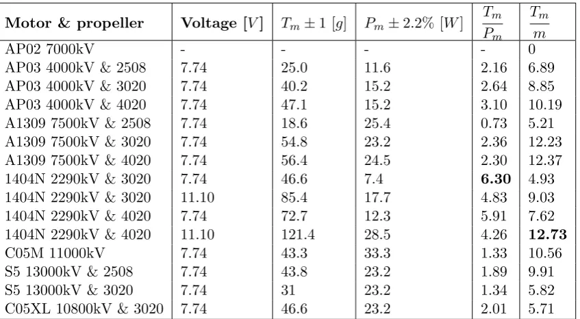
Static experiments
In Table
2.2
for each motor and propeller combination tested, several results are shown. These
are the maximum thrust for a given voltage, the power consumption at maximum thrust, the
thrust to mass ratio and thrust to power ratio. The thrust has been indirectly measured with
an 6 DOF force and torque sensor from ATI (Mini40E). During all experiments the commercial
Electronic Speed Controller (ESC) was used. For a complete overview of the test setup, please
refer to Test Plan - Iteration 1 - 16/04/2014.
The torque measured is used to compute the thrust in grams with the following equation:
T
=
τ
m·
1
l
arm·
A
N toGram[
g
]
(2.1)
with
l
armbeing equal to the distance between the axis of the motor and the center of the
transducer (75[
mm
]).
A
N toGramis equal to 1000
/g
, where g is the standard acceleration of
gravity(9.80665 [
m/s
2]). In Figure
2.1
the thrust as function of time is shown for one motor
and propeller combination to illustrate the measurement data acquired.
The power versus thrust curve of each motor propeller combination is added as attachement to
this report.
For each motor and propeller combination a curve has been fitted to the acquired data. In
Figure
2.2
, for the motor and propellers combination for which a power curve could be fitted,
the result is shown. In most cases 5 different thrust levels are used to fit a curve. However for
[image:17.595.132.465.238.396.2]Chapter 2. Measurement results
Motor & propeller
Voltage [
V
]
T
m±
1 [
g
]
P
m±
2
.
2% [
W
]
T
mP
mT
mm
AP02 7000kV
-
-
-
-
0
AP03 4000kV & 2508
7
.
74
25.0
11.6
2.16
6.89
AP03 4000kV & 3020
7
.
74
40.2
15.2
2.64
8.85
AP03 4000kV & 4020
7
.
74
47.1
15.2
3.10
10.19
A1309 7500kV & 2508
7
.
74
18.6
25.4
0.73
5.21
A1309 7500kV & 3020
7
.
74
54.8
23.2
2.36
12.23
A1309 7500kV & 4020
7
.
74
56.4
24.5
2.30
12.37
1404N 2290kV & 3020
7
.
74
46.6
7.4
6.30
4.93
1404N 2290kV & 3020
11
.
10
85.4
17.7
4.83
9.03
1404N 2290kV & 4020
7
.
74
72.7
12.3
5.91
7.62
1404N 2290kV & 4020
11
.
10
121.4
28.5
4.26
12.73
C05M 11000kV
7
.
74
43.3
33.3
1.33
10.56
S5 13000kV & 2508
7
.
74
43.8
23.2
1.89
9.91
S5 13000kV & 3020
7
.
74
31
23.2
1.34
5.82
[image:18.595.75.499.70.303.2]C05XL 10800kV & 3020
7
.
74
46.6
23.2
2.01
5.71
Table 2.2: Measurement results of all motor and propeller combinations. AP02 wouldn’t start
while both S5 and C05XL reached a too high current and thus the maximum voltage (PWM)
has not been applied.
C05M only two are used as it wasn’t able to start well with a propeller attached. If this was
due to an defect motor is unknown. For both the S5 and C05XL also two levels are used as the
current was becoming too high (inefficient and reaching maximum allowed current).
2.2. Static experiments
0
50
100
150
200
250
300
−10
0
10
20
30
40
50
T
h
ru
st
[g
]
Time [s]
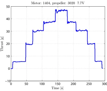
[image:19.595.127.470.87.377.2]Motor: 1404, propeller: 3020 7.7V
Figure 2.1: Measurement data of one motor and propeller combination. Illustrating the
mea-surement method used.
0 20 40 60 80 100 120 140
0 5 10 15 20 25 30 35
Thrust [g]
P
ow
er
[W
]
AP03 3020 7.7V AP03 4020 7.7V 1404N 3020 11.1V 1404N 3020 7.7V 1404N 4020 11.1V 1404N 4020 7.7V 1309 3020 7.7V 1309 4020 7.7V C05XL 3020 7.7V S5 13000Kv 3020 7.7V C05M 3020 7.7V OC
Figure 2.2: Power versus thrust fit of each motor and propeller combination
[image:19.595.77.514.461.730.2]Chapter 2. Measurement results
2.3
Step response
In Figure
2.3
a step response of the 1404N and AP03 motor is shown. For the step response
of the 1404N motor System Identification Toolbox is used to estimate the transfer function. A
4th order transfer function was fitted which has the best fit of 96.44 %.:
T hrust
voltage
=
1528
s
4+ 6
.
569
s
3+ 42
.
61
s
2+ 129
.
2
s
+ 198
.
2
(2.2)
p
1 &
p
2 :
−
1
.
06
±
4
.
92
i
(2.3)
p
3 &
p
4 :
−
2
.
22
±
1
.
70
i
(2.4)
Note: a 5 Hz low pass filter in the force/torque sensor was applied.
0 0.5 1 1.5 2 2.5 3 3.5
0 10 20 30 40 50 60 70 80 90 100
Time [s]
T
h
ru
st
[g
]
[image:20.595.122.477.279.613.2]AP03 step 7.7V 40-60 PWM 1404 step 11.1V 0-120 PWM
Figure 2.3: Step response of 1404N motor from standstill to full throttle and of AP03 from 1/3
to 1/2 throttle.
2.4
Measurement accuracy
2.4.1
Thrust
The resolution of the ATI Mini40E transducer is specified as 1
/
4000 [
N m
], while for accuracy
of the torque measurements only the typical gain error over temperature (deviation from 22
◦C
)
is specified:
2.4. Measurement accuracy
±
5
◦C
: 0
.
1%
±
15
◦C
: 0
.
5%
The analog signal is digitalised by a 16bits ADC in the NET F/T box of ATI that enables it
to be interfaced via Ethernet. Also the NET F/T box is used to apply a 5 Hz digital low pass
first order filter as for the measurement results in Table
2.2
only the low frequent component is
necessary.
Assuming
l
armand
A
N toGramare correct, given the typical gain error and equation
2.1
, the
thrust has an typical error of 0.1 %. However, as can be seen in Figure
2.1
, the thrust varies
over time with roughly
±
1[
g
].
2.4.2
Power
During each step in Figure
2.1
the DC current was measurement with a Fluke 175 True RMS
multimeter which has an specified accuracy of
±
1% [Fluke(2001)]. During measurement,
espe-cially when the motors were spinning at a high RPM, the DC current fluctuated with roughly
±
2% max. The voltage was measured with the same Fluke 175 multimeter. The multimeter
has an voltage measurement accuracy of 0
.
15%. Given the fact a relative light load is applied
to the 300 [
W
] power supply and by measuring the voltage under load, it was concluded that
the effect of an varying voltage on the power consumption can be neglected. Assuming the
uncertainties are uncorrelated the maximum deviation in computed power becomes 2.2 %.
Please note that the computed power is also due to the losses that occur in the motor controller.
The power consumption due to the idle current (motor not running) has been found to be
negligible (0.1 [
W
]).
Chapter 3
Multi-rotor alternatives
In this section the multi-rotor alternatives discussed and weighed using a weighing matrix. In
order to make a profound choice, the criteria need to be determined. These criteria originate
from the user requirement and the results from the feasibility study. After the introduction of
the alternatives the these criteria are determined after which they are applied in a weighing
matrix in Section
3.4
.
3.1
Alternatives
From the results of Chapter
2
, eight alternative configurations have been composed. These are
shown in Figure
3.1
. Four alternatives use the 3020 propeller, while the other four use the 4025
propeller. This difference is expressed in the naming: 107-XX-XX respectively 127-XX-XX.
The second part of the name list the number of battery cells it operates on. The 2S variant
uses a two cell battery while the 3S variant uses a three cell battery. The voltage respectively
is 7.4 [
V
] and 11.1 [
V
]. The last difference is the motor that is being used. LP stands for an
motor with a low power consumption, but has other disadvantages such as size and weight.
MP stands uses a motor with medium power consumption while HP stands uses motor with
an high power usage. To conclude, each alternative uses an different class motor, each with its
own disadvantages and advantages.
The flight time is calculated when everything is running at full power and in case a gumstix
and two cameras used. The hover time is also calculated in case a gumstix and two cameras are
used. The thrust to mass ratio is defined as the maximum thrust divided by the mass of the
multi-rotor
without
payload. Thus without gumstix, camera etc. The mass is again the mass
of the multi-rotor without payload. The mass ratio
R
mis also defined for the case without
payload.
Several comments need to be made about the component choices:
Reducing flight time, by reducing the size of battery, also reduces Rm, but does increase
the thrust to mass ratio and the payload.
If an high
R
misn’t necessary, reducing battery size and thus flight time, significatly
increases the thrust to mass ratio.
3.2. Derivation of weighing criteria
Power consumption using 2S (7.4V bat)
Low Medium High Using 3S (11.1V battery)
. 107-2S-LP 107-2S-MP 107-2S-HP . 107-3S
Size (mm) 107x107 107x107 107x107 Size (mm) 107x107
Flight time (min) 6.2 6.7 5.6 Flight time (min) 8.6
Hover time (min) 9.8 14.9 11.5 Hover time (min) 19.5
T/m 2.0 1.7 2.1 T/m 2.5
mass (g) 93.8 94.2 102.9 mass_empty (g) 136.8
Payload T/m=2 -1.6 -14.8 5.7 Payload T/m=2 33.0
Payload T/m=1 91.6 65.6 115.3 Payload T/m=1 203.8
Rm 5.9 16.7 19.0 Rm 10.5
. 127-2S-LP 127-2S-MP 127-2S-HP . 127-3S
Size (mm) 127x127 127x127 127x127 Size (mm) 127x127
Flight time (min) 8.2 6.0 5.3 Flight time (min) 10.3
Hover time (min) 17.3 11.0 12.0 Hover time (min) 25.8
T/m 2.3 1.6 2.0 T/m 2.3
mass (g) 124.2 102.5 113.2 mass (g) 210.2
Payload T/m=2 20.2 -23.1 -1.4 Payload T/m=2 31.6
Payload T/m=1 165.6 57.3 111.4 Payload T/m=1 274.4
[image:23.595.121.478.74.364.2]Rm 9.0 18.2 20.8 Rm 18.0