New calibration techniques for one port measurements using a computer corrected network analyser

A Thesis Submitted for the Degree of PhD at the University of Warwick

http://go.warwick.ac.uk/wrap/73386

This thesis is made available online and is protected by original copyright. Please scroll down to view the document itself.

NEH CI~LIBHATION TECHNIQlJES for ONE-PORT MEASUREHENTS using a Cm-WUTER-CORr"lECTED NETI'lORK ANALYSER

by;

. E. F. da SILVA, H.Se., C.Eng., M.I.E.l~.E.

A Thesis submitted for the Degree of Doet.or of Philosophy

..

School of Engineering Science university of l'1arwick

West Yorkshire, LS23 7BQ

www.bl,uk

BEST COpy AVAILABLE.

( i)

CON'rENTS

Chap'ter I PAGE

A

BRIEF REVImi OF SOHE REFLECTION COEFFICIENT' MEASUREHENT SYS,)~EHS

1:0 Introduction 1

1: 2 The Reflection Bridge 7

1:3 Time Domain Reflectometry Measurements 10

1: 4 Swept Frequency Slotted Line Heasurements 15

1: 5 Directional Couplers 18

1: 6 Conclusions 21

1:7 References 23

.Qhapte'r

II

THE THEORY OF THE MEASURING SYSTEH

----2:0 2:1 2:2 2:3 2:4 2:5 2:6

Chapter

:rg

Introduction

The Theory of Reflectometer Measurement Reflection Coefficient

Directional Couplers

The Measurement Uncertainty of Incident and Reflected Power

Conclusions References

THE HEASURING SYSTEM (Hardware)

3:0 3:1 3:2 3:2.1 3:2.2 3:3 3:3.1 3:3.2 3:3.3 3:3.4 3:3.5 3:4 3:5 3:6 3:7

J~ntroduction , , : j " , ' . . Description of the Measuring sys't~T .' .

The Signal Source Bloc]e

Frequency stability 2:~

'."

The Importance of Source Ma tell," ,,~ <'\ Cl10ice of the Reflectometer ...

Directivity

Vol tage Standing 'Vlave Ratio (VSWR) Frequency Range

Coupling Coefficient Transmission Loss

'I'he Det.ection and Indication Block System Accuracy

Chapter IV

lmCOH ...

'lliGTt~D REFLECTOHETER HEASUREHENT

4:0 4:1 4:2 4:3 4:4 4:5 4:6 4:6.1 4:7 4:8 4:9

Chap_tg?; ..

y

Introduction

The Limits of Reflectometer Accuracy Directivity Error

Source Mis-Match'Error '

The Combined Heasurement Errors

The Effects of Adapter/Connect.or Errors An Alternative l1ethod of Specifying

Reflectometer Accuracy Application of Error Equations System Accuracy

Conclusions References

REFLEC'l'OHETER CORRECTION HETHOD~

5:0 5:1 5:2 5:3 5:3.1 5:3.2 5:4 5:4.2 5:4.3 5:4.4 5:4.5 5:4.6 5:5 5:5.1.1 5:5.1.2 5:5.1.3 5:5.1.4 5:5.2 5:6 5:7 5:8 Introduction

The Elements of the Error Correction Model Correction Me-thods Using the Invariance of the Bilinear Transformation Cross Ratios A General Review of One-P ort Reflectometer

Error Correction . Theoretical Error Model

Practical Error Model

Specific Calibration Procedures

The Three Short Circuits Correction Method 'I'he Short/Offset Short/Matched 'l'ermination

Correction Nethod

The Three Open Circuit Correction Method The Three Identical Non-1-iatched

'l'ennination Correction NeLhod

The Short/Offset Short/Open Circuit Correction Nethod

The Four Termination Correction Methods Difficulty in Specifying

Calibration Lengths

Difficulty in Defining the Calibration Terminations Changing the Po si tion of the

Heasurement Plane Construction Problems

The Four Termination Correc·tion Methods 'rhe Evaluation of the Reflection

6:0 6:1 6:2 6:3 6:3.1 6:3.2 6:4 6:5 6:5.1 6:5.2 6:5.3 6: 5.4 .

6:5.5 6:5.6 6:6

6:7

6:8

ChaP.-teE,

V:g;

(iii)

Introduction

The Three Short Circuits Calculator P rograrrune

The Three Shorts Sigma V P rogramlne for Hanual Use

The Four Shorts Sigma V Programme for Manual Use

The Four Shorts (Single Precision) Programme for Manual Use on the

Sigma V Computer

The Four Shorts (Double Precision) Prograrrmle for Hanual Use on the

Sigma V Computer .

The Four Unknown/Reference Short Termination for Manual Use on ·the Sigma V Computer

The Aut~mated Computer Correction Programme

Basic principles

Interface Between Operator and Computer The Control of the Signal Frequency Measurement, storage and Calculation

of Data Reproduction of Results Supplementary Tasks

The Automated Progra~me for the Three Short Circuits correction Hethod Conclusions

References

THE FABRICATION OF TEST A:ND C]\LIBRA'l'I.ON PIECES

7:0 Introduction

7: 1 General Details of the Calibration

7:1.1 7:2 7:3 7:4 7:5 7:5.1 7:5.2 7:5.3 7:5.4 7:5.5 7:6 7:7 Standards Choice of Off set Lengt.hs

The 7mm Short Circuit Co-Axial Calibration Pieces

3mm Short Circuit Calibration pieces Construction. of the Open Circuit and Reference Short CO-Axial Calibration

Standards

Fabrication of Microstrip Circuits Maskroaking

Photo-Li thography substrate preparation

£hapt?-r

vrrr

PRACTICAL PROBLEHS IN COJ'1PUTER CORREC'fED MEASUHEMENTS

8:0 8:1 8:2 8:2.1 8:3 8:3.1' 8:3.2 8:4 8:4.1 8:4.2 8:5 8:6

Ch1?-pter T~

FESUL'rs OF

E~crrION

9:0 9:1 9: 1.1

9: 1. 2

9:1.3 9:2 9:2.1 9:2.2 9:3 9:3.1 9:3.2 9:4 9:5 9:6 9:6.1 9:7 9;7.1 9:7.1.2 9:7.2 Intrcduction

A Drief Review of the Measurement Equipment

Sources of Errors in Automatic Network Analyser

The Instability (Non-repetlotivc) Problem Practical Difficulties in Measuring

Large Reflection Coefficients; Amplifier Limiting Problems Modification of Error Scattering

Parameters

The Effect of the Multiplication Factor

"k" on Line Propagation Properties Preliminary Computer Corrected

MeCl.8urements

A Manual Correction Test An Automated Correction Test Conclusions

References

MEASTJREMEN'rs (incl,!ding accur_<?:~'y) USING THE l'-!-r::W

COEFPICIEN'l' CORREqTION MEASURgHENT SYSTEM~

209 209 213 213 215 216 218 218 218 220 220 226

Introduction 227

Measurement Results Using the Three Short

Circui t Correction Hcthods of section 5: 4.2 228 Measurement of a Short Circuit 228 Measurement of a Matched Load 233

Errors in Correction 233

Neasurements Results Using the Four Short

Circuits Correction Nethod of section 5:5 233 Measurement of a Sliding Load Termination ~33

Meaf3urement of

a

Short Circuit 237 Measurement Results Using the Four Unlmown

Ter.TIlinations, and Reference Short Hethod

of Section 5:5 238

Measurement of an Attenuator Terminated

by a Short Circuit 238

Measurement of a Short Circuit 243

Co~parison of Results Using Different

Correction Techniques 243

Accuracy of Measurements 247

The Practical Aspects of Correction Accuracy 252 Avallabili ty of }feasurement Standards 253 General Procedure Used for Verifying

System Aecuracy 254

Accuracy of Measurements Using the 3-Short Circuit Correction Method of section 5:4.2

and the Cornpnter Programme Described in

section 6: 5 258

Measured Accuraci0.G of the Heans 260 Accuracy of Meal:~urements Using the 4-Short

,Circuit Correct.ion Nethod of section 5:5 and the Computer Programme Described in

(v)

.Qh;:pt.~r IX • ~. Continuation

9:7.3 9:8 9:8.1 9:8.2 9:9 9: 10

Cha12ter X 10:Q 10:1 10: 1.1 10:1.2

10 ~ 1. 3

1012 10:3 10:4 ~endice~ 11:1 11:2 111 3 11:4 11:5 1116 11:7 11:3 11:9 11:10 11:11

Accuracy of Measurements Using the

4 Unknovm Terminations and a Reference Short Circuit Correction Method of Section 5: 5 and the Computer Programme of Section 6:5

Comparison of Results for the Three

New' Types of Measurements

Comparison of Results at 4 GHz

Comparison of Results at 6 GHz

Conclusions References

Final Review

Achievement of Objective

The Three Short Circuit Correction Method The Four Short Circuit Correction Method The Four Unknmvn Termination/Reference

Short Circuit Correction Method Final Conclusions

FutL/re Work References'

The Usefulness ·of the Bilinear Transformation

Bilinear Tra~sformations of scattering Parameters

The Bilinear Transformation of a Circle in the Complex Plane 'l'he Invariancc of the Bilinear

Transformation Cross-Ratio Applied to Micro'iTave Analysis

Programme for Reflection Coefficient Correction Using the 3 Short Circuit Method of Section 5:4.2

Hannal Programme Using Sigma V Computer for Reflection Coefficient Correction Using Three Short Circuits

Hanual Progranune Using Sigma V Computer for Reflection Coefficient Correction Using Four Short Circuits

Hanual Programme (Double P recision) Using sigma V computer for Reflection

Coefficient Using Four Short Circuits Manual P rograITh'110 Using Sigma V Computer

for Reflection Coefficient Correction

U sing Four Unk.nown Termina·tions and C!

.Appendix 12 - Publications

12:2

12:3

Calibration of Hicrowave NetworJc Analyser for Computer Corrected S Parameter Measurements

Calibration of an Automatic Network Analyser Using 'rransmission Lines

of UnknOivn Impedance, Loss and Dispersion

. Calibration Techniques for One Port Measurements

*

* *

*

*

* *

*

* *

PAGE

325

328

(vii)

ACKNOHLEDGEHENTS

I wish to eA~ress my gratitude to Professor J.A. Shercliffe, Chairman of the Department of Engineering Science, and Professor J. Douce, Head of the Electrical Department of the University of War.vick for the facilities provided for conducting these

investigations •

•

This work was supervised by Dr. M.le }fcPhun to whom I am most grateful for his technical and friendly guidance dud.ng the past years and for his constructive comments in the preparation of this manuscript. Thanks are also due to }ir R • .l\nderson of Lanchester ~olytechnic for many . constructive discussions.

In the Department of Engineering, I am indebted to

Dr. H.V. Shurmer and in particular to a former graduate student Dr. N. Hosseini who offered most valuable advice in the writing of the automated programmes. Thanks are also due to }fr A. BUlne, Mrs K. Stoneman and }fiss L. Harvey of the Departmental Computer section.

Acknowledgement is also made to the Science Research Council for partial financial support.

Finally, I would like to thanlf. my wife Ann, who endured the many months of "wido·whood" whilst this thesis 'vas being finalized.

ABSTRACT

The thesis presents three ne,,: computer correction methods for me<::.suring immittanccs and reflection coefficients using an automatic network analyser. 'I'he first correction method

called the "Three Short Circuit Correction Hethod" was invented to overcome the 'difficulty of measuring components embedded in microstrip or in conf~ned environments where sliding nlatched terminations required by normal correc·tion m8thods cannot be used. With this nevT method, error correction is carried out based on'calibration measurements produced using three unevenly spaced short circuits. This method was subsequently published in the I.E.E. journal "Electronic Letters" of 22nd March, 1973.

The second correction method using four evenly spaced short circuits '\vas introduced t.O overcome the difficulty of accurately specifying electrical lfmgths in microstrip or

in

a transmission line with non-hmnogenous medium. The third correction m~thod 'I-laS evolved to overcome the practical

difficulties of constructing good short circuits ,dthin micro-strip lines. with this method, direct knm\Tleug0. of the

terminations of the calibration stcmdardG is Ul1!1.ecessary. Rigorous theoretical derivations for the last two correction methods have been published in the I.E.R.E. journal "Radio and Electronic Engineer" issue of }fay, 1978. Detailed

n1Gasurcment results and comparisons of the different types

of correction measurements have been published in the

( ix)

'I'be last

t.wo

correction methods also provide a means

of measuring the attenuation and phase changes of transmission

lines, and ·the effective dielectric constant of a

non-homoger.ous line may be calculated if its physical length is

k.."lown •

Comparative measurements carried out using the new

correction systems as opposed to the older established

correction syst.ems are included in this thesis. They agree

most favourably.

Results obtained using a.ny of the new correction systems

have s!1own that measurement accuracies of

+

0.5% with a

confidence level of 99% are attainable. These results have

been con finned by statistical data obtained from repeated

meas'J.rements

(100

in some cases) of an accurately defined

test standard.

DECLARATION

Unless othel\vise credited, all the theoretical and practical work described in this "thesis is my own.

This worlt has not been submitted at any other university or institution although some parts of this thesls have been

published in tec1mical -journals.

I

(xi)

PREFACE

Overall Aims

The overall aims of this thesis evolved from necessity. 'rhe necessity arose when a team of researchers at t11e

University 'of Warwick were invest.igating the applicution of lumped components, (transistors, resistors, inductors and capacitors) for use at microw·ave freqtlencies. As these elements were constructed, i t was found that there w·ere no convenient means for accurately charaC?terizing these devices. The author trlen undertooJc the tas}~ of remedying this deficiency. This worle proved to be a far greater tasle than originally

a.nticipated and the ·author's original research on inductors had to be cast aside in favour of the measurement problems.

Investigati.ons originally began with the then currently used rapid measurement techniques for evaluating immittcmces

a.nd after this survey (ChapterI), i t ,·,ras decided that the reflectometer. "lQuld be used. The principles of the reflcct.o-meter was subsequently investigated in Chapter II. The

peripheral equipment associatc:·d with i t were investigated in Chapter III.

For measurement accuracy, inherent measurement errors must be recognised and el,iminated· if possible. Hence, the errors associ.ated with reflectometers had to be investigat.ed. TIle two main errors, directivity and sourca match, have been discussed extensively in Chapter IV. A study of these

equipment ei~rOL'S revealed that they are extremely difficult t.o elil!1il1d.1:-I~ over large measurement bandwidths. Hmvever I

described in Cha.pter V. These correction methods have now been publi Ghed. Sofb-rare correction methods require consider-able mathematical manipulation of complex numbers and five manual computer programmes and two automated programmes had

to be written. These have been described extensively in Chapter VI.

The calibration procedures required the construction of several calibration pieces SUdl as short-circuits, off-set

short circuits etc. These have been shown in considerable detail-in Chapter VII.

The determination of the suitability of the equipment for use ill computer correction measurements has been

established in Chapt.er VIII.

The results of some measurements carried out with the new correction systems are shown ill Chapter IX. p.. substantial purt of this lengthy chapter has been devoted to establishing the accuracy of the corrected measurements. To minimise

random errors, many measurements (up to 100 in some ca.ses) have been carried out to detennine the accuracy of the measurement procedures.

The final conclusions of the thesis are summarized in Chapter X. Suggestions for further work has also been included in this chapter.

Appendices 11.1 to 11.10 contain details of some fundamental principles used throughout the thesis whilst appendices 12.1 to 12.3 include the published papers that have result.ed from this work.

- 1

-CHAPTEH I

A BRIEF REVIEW OF SO}ill REFLECTION COEFFICIENT MEASUREHENT SYSTEMS

1:0 Introduction

The purpose of this thesis is to establish new computer corrected measurement procedures for determining the

irrunittances of lumped components (-transistors, resistors, i.nductors, capacitors etc.,) used at microwave frequencies. The necessity for this thesis arose when

a

team of research-· ers at the Uni versi ty of l'larwick were engaged in the

application of lumped components. As thcr;e fundamental devicer:; were constructed, it was found tha.t there "\'las no convenient means for accurately characterizing the devices. The inability t'o characterize these devices affected the

author's work most profoundly as.he was then involved in the construction and application of lumped inductors for micrmvave use. The test jig for measuring these inductors

(Figure 1.1) had already been built and specimen components (Figure 1.2) had already been constructed. The same

problem "\vas also experienced by fellow researchers D. Nichie in his measurement of capacitance and A. Kwesah in his

characterization of transistors.

The cl.ifficul ties shared in common "d th these fellow researchers were that computer correct.cd measurements using reflectometers could only take place at a reference plane where calibration standards such as a sliding load could be used. Hence if a device \vas embedded in a dielectric

medium some dist~nce uway from this reference plane, then only the t.rans.ferred immi ttancc i.

C!.,

device im.-ni ttance transferred t.hrough a length of transmission line could be

F:igure 1.1: Test. J'ig designed by the author for the

measurement of lumped components.

Fi9ure 1.2:

'

.

- -_.

__

.. - ---- . - - - _ . - - -~- ... _-.. *._---_ .... _ ..

A typical lumped tuned circuit const.ructed by the author on a 10 x 10 mm substrate for

- 3

-'1'his deficiency had to be resolved and the author then abandoned his own 1vor]{, on inductors and und8rtook the tasle of providing a solution t.o the measurement dilenuna. Hm:ever, before thi s tasle could be carried out, a survey of the many different methods of measuring irnmittances had to be invest-igated.

This chapter presents a brief review' of some of the more commonly used systems for measuring irmnittances using

reflection coefficients methods. The measurement systems chosen for discussion are the Rhotector (Section 1:1), the six Element Reflection Bridge (section 1:2), Time Domain Reflectometry (Section 1:3) and Swept Slotted Line Frequency l1easurements (Section 1:4), Directional Coupler (Section 1:5).

The above methods were selected for investigations chiefly because of the ease of measurement over wide

frequency bands. Many other methods of measuring reflection coefficients are also Y~own e.g., Deschamps Method etc., and a comprehensive explanation of these methods may be obtained from tbe excellent series of books on rnicrm'lave measurements by Sucher and Fox (Reference 1.1).

1:1 The Rhotector

Figure 1.3 Input Voltage

Bridge Output Voltage

Rectified J..

detector output voltage.

Siveep Frequency Generator

The Rhotector (ref.

1.2)

is a reflection coefficient measurement device based on the '~heatstone Bridge principle. Its corifiguration is shown in figure 1.3 where Z3 andZ_{4 are} equal resis·tances (usually 50 ohms). Zl represents the impedance to be measured and Z2 is tl")e reference impedance.

l'llicn the bridge is balanced, the bridge output voltage (V

_o)

is zero and the detector output voltage (V

_n)

is also zero. When the bridge is unbalanced, i.e., ZI f- Z2 an out-put voltage

Yo'

causes the R.F. diode detector to produce a voltage YD'

The rhotector is constru.cted with a 50.n. coax.ial

measuring port and is supplied with a kit of 8upp1cmentar.f coaxial loads having "volt<1ge standing wave ratios (VSHR) of

1.0, 1.5,

2.0, and 3.0. For wide band measurements, a

s.·vleep signal generator is connected

tc;>

the input terminal s and the detector output signal is nonnally connected to an oscilloscope whose time base is synchronized ·to the s"V,Teep frequency. Z2 is externally terminated with a load of VSWR

=

1 and Val~E.~S of Zl using the calibration st.andards

are used to calibrate the appropriate VS\~R t S on the display

oscilloscope. The device to be measured is then inserted in place of tl1.e calibration stan9ards and the VS-vR displayed is interpolated.

Referring to figure 1.3 i t is seen tha't provided the

diode detector does not load the bridge networ}.::, then

::. V

z,

-

_'7

J

z%.~

5

-and since Z3 :: Z4 = Z by construction and if Z2 is chosen to be Z, then

y'~,

\1

+}

·

....

1.1

The above measurements are usually carried out at low .si.gnal·po"iers (-10 aBm) in ""hieh case the diode detector characteristics may be assumed to be square la",' i. e, , . IDIODE' :: k vin (DIODE') where 1{. == diode constant.

Th!? detector output voltage (V D)

where

1\ ::

Diode Load Resistance hence, sUbstitut.ing in equation 1.1

v~

• • • • •

1.2

If l':---Rl.:.. is defined as

K

then equation 1.2 becomes

4

·

..

,

.

1.3

+"'Z-The voltage standing ... ave ratio (VS\~R) is related to the reflection coefficient ( " ) by the expression

r=

and substituting in equation 1.3 yields

V;p

=

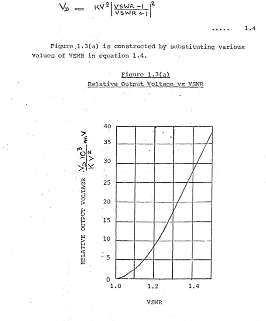
[image:21.595.62.539.37.811.2] [image:21.595.30.563.167.808.2]

• • • • •

Figure .1. 3( a) is constructed b¥ snbs,ti tuting various valuca of VSNR in equa.t.ion 1.4.

Figure 1. 3{

a.l

RE~lati ve Ou.:9:2.ut Vql taqe vs VSNE

~

~~~

0>

;I~

~

f.iI 0

fS

..

~

0

:>

b

~

p 0 f.iI

:>

H

8 ~ H

~

40

35

30

25 1

-20

*5

10

-.-, 5

~

o

1.0

.

.

L

----

--/

.

V

/

/

V

/

I

V

--I

,/

1.2

1.4

VSl'lR

7

-A more detailed analysis of the Rhotector may be found in reference 1.2.

The rhotector is a relcA.tively simple and useful device for measuring re~lection coefficients over wide frequency bands and it is an ideal production test instrument as i t is relatively robust. I t 'vas not selected as the main measurement system

because:-1: Only the modulus of the reflection coefficient is measured.. Phasor values cannot be obtained.

2: The reflection coefficient measured is dependent on t.he ac"curacy of the !:lain calibration tes'!:. standards.

3: The reflection ~oefficient measured is directly proportional to the square of the value of the input voltage (equation 1.2) and over a ,vide frequency band of measurement the input vOltage may vary considerably.

4: The detector output voltage is not linearly related to the reflection coefficien·t or VSWR

(figure 1.2). Furthermore, this output is subject to the temperature vagaries of the diode character-istics.

5:

The signal applied to the device under test

(ZI)

is always less than the generator applied voltage and could lead to poor signal to noise ratios when low reflection coefficients are measured.

1:2 The RQ,flp.ction Bridge

Figure 1. 4( a}

The Six Element Reflection Bd.d~

r---~izol---~--V D

n

'1

Impedance

The reflection bridge is a six-element bridge which assumes the configuration shmm in figu:r-e 1.4(a). This neb·:orlc configuration has the grea"t advantage in that the detector output voltage (V

_o)

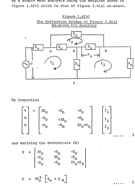
is directly proportional to the reflection coefficient. The network can be analysed

[image:23.573.48.518.142.800.2]

by a simple mesh analysis using the notation shown in figure 1.4(b) "i-rhich is that of figure 1.4(a) re-draHn.

By

•

Figure 1. 4(hl

The Reflection Bridge of Fiaure 1.4i.~1

Re-dra\·m for Analysi s

B

c

fnspection

V

=

3Z

0 -Z 0 -Z 0

0

_-ZO

_+3Z

0

-Z

0

0 -Z

-z

" 220+Z ...

0 0 < ...

• • • • •

and defining the determinate (D)

D

=

D

=

-z

_o

3Z

o

-z

_o

• • • • •

1.5

- 9

-The detector ou·tput voltage (V

_{n )}

is

VD

using Cramer's Rule to solve for I2 gives

12

=

3Z

_o

V -Z ₀ -Z

0

-z

0

0

. -Zo 0 _{2"Z{"Z .}

. _1

•

~

[ 3VZo2

J

/

I2

+

VZOZ OX D

and

I.,

₌

3Z

0 -Z

..) 0

.-ZO 3Z

0

n

-z

. 0 -ZO

•

13

~

_{[4 V Zo 2J /}

D

• •

Combining equatiors 1.6, 1.7, 1. [: and 1.9,

or

v

0

=

V

[z:.c ..,.

Z 0]

8

[z.~

+

zoJ

v

[rJ

8

where

r

=

_{- - -}

Z:.:, - Zo as shm·m in equation 2. 19.

z"

+

Zo

·

..

.

.

.

1.7

·

.

.

.

.

1.8

· .

. . .

1.9

••••• 1.10

Hence the output voltage V 0 to the reflection coefficient ~

In;~:recr~ ~ (ReF' l . .3) '~lISIZl>.

is directly proportional • PA.e","~ 1"" ...

1\,

A L\~EAil

The insertion loss of the bridge is high, the out.put voltage being ~:me eighth of the open circuit generator voltage or ~ of the voltage that would be delivered by the generator if i t ,,;as correctly terminated by an impedance

Zo

in place of the bridge. Thus the insertion loss is

12dB.

Practical realisations of the bridge circuit have losses slightly greater than this. This high insertion loss has t.he adv·antage that source mismatch error (cectio:1 4 ~ 3) is reducGd but.it also causes reduced signal level to the device under test.

The greatest: problem "d th the bridge described is that aball.:t.n;· must. be provided for the R.F. Source or the detector. This condition is most difficult. to satisfy where microwave

frequencies operating over several octave bandwidths are desired. If a crystal detector is placed across the

detector load such as in the Wil tron Autotest.er (reference 1.4) . the baluns problem is overcon1c but then only the magnitude

of . the reflection coefficient

I

r

I

will be obtained and

many of the disadvantages common to the Ehotector (section 1: 1)

'vill be evident.

A

more detailed analysis of this bridge may be found ip references 1.3 and 1.4.

This bridge was not favoured for t:hc measurement of complex reflection coefficients for the' reaSOnf.l discussed in sections 1: 1 and 112. in spite of its higher directivity. The problem of directivity errors will be discussed fully in

section 4:2.

~ Time Domain Rpflectorn.etry Neasurement.~

Time DOmain,. Reflectometry employs a pulse generator

,

[0

0

..

J

0 0

- 11

-If the terminating impedance is not matched to the line, then reflection occurs. Both the incident and reflected steps are monitored by an oscilloscope at a fixed point.

[image:26.577.35.517.45.777.2]

STEP

Figure 1.5

. Bloc1~ Diagram of a Simple Ti.me Domain Reflectomet£Y SYsts~

OSCILLOSCOPE

fEi

BRIDGED

rr

UNKNOWN

GENEHATOR TEE IHPEDANCE

--The following can be deduced from an intelligent comparison of the incident and reflected ·step waveforms.

11 Any discontinuities in the line can be located by virtue of the propagation velocity of the step

function and the time (measured on th~ time base of the oscilloscope) required for the reflected voltage to return. This feature is 'extremely usefUl for locating poor connections etc., within a system.

2: The waveform of the reflected wave from any

dis-continuities or terminations is most valuable for it reveals both the nature and the magnitude of the mismatched 'termination.· Eight ideal oscilloscope displays o~ this nature are shown in. figures 1.6 and

1.7. TheEG diagrams have been taken. from reference

TDR Displays for Typical~oags

---.

0 . - - - 0

ZL ---:;;. (P. ) _{OPEN CIRCUIT TERMINATION (ZL = 00)}

~J

-E.

1.

0 - - - 0

0 - - - - ,

>

(D) -SHORT CIRCU!'!' TEIDUNA'I'ION (ZL

=

0) o

z

_{I ..}

-->

(C) LINE TEPJUNATED IN ZL = 2Zo

~.

;_0-ZL

-->

(D) LINE TERHINA'l'ED IN ZL ₌ ~'Z _{2 0}

(";

(,

--SERIES

R-L

13

-Fignre

1.7

Q8cl110sco~p'isplays for Complox Load Im}20danc€s ZL

(

R-2 R-l

-V)

.[. (I + _ Q . ) + ( I - _ _ 0) e T

( I R+l R+Z

o 0

WHERE T" __ L _ R+£o

~--+.-t--+

t

o

R-l

(I + -_OJ E· R+Z I

T

0

z ... ·

_L

I

R

L

R

: I

n

Z-+

L C

These (-?xprE!ssions may be derived by recalling that the reflection coefficient (~ ) is given by:

ER

E'

..

=

1.

••••• (Ref 1.5)

where E

R

=

Reflected Waveform

EI

=

Incident S·t.ep Waveform

~L

=

Terminating Impedance

Zo

..

Characteristic Impedance of the

'l'ransmission Line.

Assuming

Zo

is real, it become only a mat.ter of simple substit.ution in the above expression to c~erive the four expressions sho\~n in figure 1.6. The waveforms for figure 1 .. 7 .can be verified by resorting to the use of Laplace

Transform i.e., w·riting the expression for \-,( s) in tenns

of the specific ZL for eac~ _.c;1. example (Zr _~.... ~ R~sL, l+r_s C' etc.) roul tiplying

r(

s) by --;;--, the transfonu of a step

Q

function of height. E. I and then transforming this product

1.

back into the time domain to find an exact expression for

ER

( t ) .

Time Domain Reflectometry was used in the development of the test jig shown in figure 1.1.

Time Domain Reflectometry

,.,as

not chosen for the main measurement system because of:

1: Difficulty in measuring "the gradients of the display waveforms accurately.

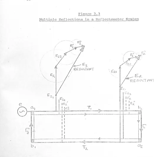
2 t N\.:~ltiple reflect.ions in a practical syst.em.

3: Relatively poor rise time of step generator at that ti.me for high frcqu.cncy wor)t ( 6 GIl )

z

4: Difficulty in observing the waveform accurately,

- 15

-1:4 Swept Frgg:L2cncy Slotted Line Neasurements

A basic block diagram of hml a slotted line may be used in s"\'lept frequency measurements is shown in figure

1.8.

Fiqure 1.8

Dlock Diagram of VSWR Measurements

Using the Sweep Fregvency Slotted Line Method

MODULATED DISPLAY

SWEEP FREQUENCY

GENERATOR t---~---~

Time Base

STORAGE OSCILLOSCOPE OR PEN RECORDER

INPUT SENSOR

fTTENUATOR

)..._----1.

~

PROBE

SLOT'rED

LINE

Ref. Signal.

Ir .

~

.~mpl. _•

,

output . signal

in dB

DEVICE ur,mER TES'r

Neasurement j.s relatively easy to carry out. The

frequency generator is set to S'tleep the desired freque:r.cy band. The device under .test is removed and a power meter is connected to the output port of the slotted line. The generator is adjusted until the desired output power e.g.,

terminaticn

e.g.,

a sliding load. One input (carriage input) of the differential amplifier is grounded and the other

input (reference input) is adjusted by the attenuator to I>roduce a sui table output e. g. , - 25dBm. The carriage input to the differential amplifier is then re-introduced and the probe penetration adjusted until the two inputs are equal,

i.e., no output from the differential amplifier. At this stage, movement of the carriage assembly on the line should theoretically produce no change in output from the

differential amplifier. In practice slight changes occur because of an imperfect slotted line and termination. The .advant:nge of using a differential amplifier lies in the fact

that small changes in input. power do not introduce large errors in VSWR measurements (reference 1.6). The output of the amplifier is then connected to a pen recorder or storage scope whose ordinate axis is initially set at its

mid-. position in order to al1mY' measurement' in ei thc~r direction. The slotted 'line terminatio!1. is then removed and the device under tes·t (DUT) is reconnected. The probe carriage on the

slotted line is slid manually to and fro over a distance (d). The distcmce (d) must exceed half an electrical ,-ravelength of the lO"'lest frequency to be measured. The resultant plot of a typical set. of measurements is shown in figure 1.9.

Fig~re 1.~

Tl'nJcal VSWRP lot of a $'v~...Qt Slottesl Line Neasurement

-·---,.---+---t----T

-.----I---I----+----t-.----t---t

• IEmax(dB

j

~-.

' - " K ..

-~----.~~

~

}-"--.I\,._n-j-·

--:;A..--=:::-..:~~:-..:::::::-=_t-=:..--!:==--:

I

~ f·---~~---+---~

({; i

~' ---~---~

12

13

14 15 16 17 18

17

-The SWR(dB) at a particular frequency is deno·ted by the distance between E_l1AX(dB) and EH1N(dB) (figure 1.9) at that particular frequency. The VE:\\fR ratio and hence the

magnitude of the reflection coefficient can be calculated in the usual manner.

A simple e~~lanation of the above procedure can be obtained by first considering operation at one frequency only. E_MAX and EMIN of this particular frequency can be obtained by sliding the carriag8 probe along the slotted line over a distance (d) greater than half a wavelength. This information will enable the.VSWR to be calculated. Phase infonnation will only be obtained in the distance through ",hich a fixed reading t e.g., E ... ..f. has moved is

l.111

lcrlOwn when the device under test at the end of the slotted line has been substituted for a reference ·termination e. g. , a short circuit. If the recorder or storage scope is

capable of recording EMAX. and EMIN in dB then since

VSvTR(dB) _{= 20 log "}

~}L~X

EMIN = 20 log

IE

Y..AX

I

I . '

-20 log J ENIN

I

it. fo1101'1s that· the d:i.fference between

I

EMAX(dB)

I

and

I~HIN(dB)

I

,.;rill yi.eld VSWR in dB. If another frequency is

chosen, E

MAX and EMIN "vi11' occui 'at different points along the slotted line. For a series of different frequencies (swept frequencies), the series of EMAX and EMIN will be locat.ed as the carriage probe is moved slm'11y along the slott.ed line and their amplitudes will be recorded. Hence the VSNR at anyone frequency can be obtained. It shoUld be noted that there is no phase information in this series

of measurements.

This type of measurement was not selected as the phase' information cannot be ea.sily obtained in theG(~ swept mear.;ure-l11ents.

1:5 Directional CaU'olers

Directional, Couplers are devices which sample a wave moving in one direction but not in the other. Such a device can be used to measure the reflected and incident waves in a measurement system and penuit the calculation of the reflect-ion coeffici.ent., The constructreflect-ion ~f a very simple directional coupler is nbm.,rn in figure 1.10 and a simplified circuit

sho1'ring the capaci ti ve and mutual inductive coupling and the irmer conductor of the coaxial line is shown in figure 1.11.

An extensive analysis of the dual directional coupler is carried out in Chapter II. The analysis carried out in this section is a very approximat2 solution and is based on that by Carson (reference 1.8) but it does demonstrate the principle of single frequency operation clearly. It also . explains why the directional coupler "Joan iJ.dcptcd as the main

device for measurement of reflection coefficients and impedances.

Fi!J..ure 1 !.LQ

Ba~ic;:s.onstruct.ion of One Type of Directional C01.lPl er

-r--'

R <

,..---\

-

-

-Loop coupled to Inner Conductor

- 19

-F:i,oure 1,11

Simplified Circuit Sho11T.ing Capaci ti ve and Nutua1 Inductive Coupling Between the loop and Inner

Conductor of a CoaxiC!l IJine Coupler,

OUTER CONDUCTOR

-~

V

R

Output

Input

Jc

L

+

V n n

End

_k-VL-~

C End

M

INNER CONDUCTOR

---1

I

By inspection of figure 1.11, it can be seen that

R V

;-~'-,-L

JWc

=

If R /<,.1- then V

R A...J jw CRY

"", JWc • • • • •

Current I in the inner conductor induces _VL in the loop. Thus,

• • •

•

•

The output volt~ge ~s

.

Vo

-_- V _R +

v

L

=

jw CHV -jw MI

• • • • •

If the coupler is designed such that

_tL

CR

= HO _{• • • • •}

1 •• 12

1.13

1.14

then equation 1.14 becomes

vo

=

jw M ( __

Y-- -

I)

RO

The voltage and current decomposition equations are

v

₌

V· _J.

+

Vr

·

.

. .

.

V. _Vr

and

I

'=

I·

-

_Ir

= J.

).

RO 1\0

•

•

•

• •

where the subscripts i and r represent the incident and reflected directions.- Thus equation 1.16 becomes

v.

+ V

V 0

=

j vtM (- l. HO r

• • • • •

1.16

1.17

1.1:7(a)

1.18

Therefore the output voltage is proportional to the reflected phasor current (or phasor voltage) because the incident components cancel when the coupler is connected as sho'Ym in figure 1.ll. If the coupler is reversed, its out-put voltage

is

proportional to the incident phasor current and the reflected components cancel. In many caSE~S, i t is not convenient to keep reversIng the coupler, and dual directional couplers, one to measure the incident wave and the ot.her to measure the reflected "lave are used. A reflect-ometer is a dual direc'cional coupler specially manufactured for good amplitude and. phase coupl:i.ng match over C\ wide

frccJ,lency band of operation.' Reflectometer design is

- 21

-In practice, the directional effect is not perfect and leads to a tl'Pe of error called "Directivity Error".

Directivity Error is investigated extensively in Chapter IV. However in spite of the errors associated with reflecto-meter measurements, this method was chosen as the most suitable because~

1: The reflectometer method provides a quick and easy method of measuring reflection coefficient and hence impedances if the reference impedance is well defined.

2& Swept frequency measurements a~e easily carried out.

3: The reflected and incident measurements carried out yield both amplitude and phase information. See equati.on 1.18 where Ir. is a phasor quantity •

. 4: Error correction systems are relatively easy to incorporate.

5: The signal loss bet"\veen the' S\veep frequency signal generator and the device to be measured can be Ie sa tha.n IdB. Thus low-pow'er signal generators can be used or alternatively larger powers can be fed to devices such as transistors if desired.

~

6: The sampling loss associated with the incident and reflected waves can be easily controlled in the initial design of the reflectometer. A commonly used coupling factor is 20dB nominally.

rrhe necessity for new rapid and computer correction systems has been established in the early par-t of this chapter. The latter p~rt of this chapter has presented a brief review of some of the various methods of measuring

investigated has several desirable properties. The Rhotector and the \AI il tron Auto tester are ideal production test·

instrUtltents, robust and simple to use for rapid magnitude measurements of reflection coefficients. Time Domain Reflectome·try locates discontinuities rapidly and Loeb

(reference 1.9) and his team have used i t most successfully in the measurement of lumped components. The Swept Slotted Line }feasurements Technique, although relatively accurate does not provide phase information. The Directional Coupler provides both amplitude and phase information rapidly and does not suffe.r from the haluns and higher loss problems

associated wi-th the reflection bridge. Herlce, the Directional Coupler was- selected as the basis for the measurement system.

'l'he remuining chapters will be devot.ed -to the application and error correction methods published by the author for the measurement of reflection coefficients and immittances using reflectometers.

23

-References

1.1 Sucher; H and Fox, J; "HandbooJc of Microwave Neasure-ments" 3rd Edition, Volumes I, II, III, John vliley & Sons J.Jtd., London.

1.2 Te10nic Engineering Co "FHO-Tector VS~~R Detector" Application Bulletin 301.

1.3 Oldfield, W. 11. "P resent-Day S:i.mplici t.y in Broad-band SWR Measurements" l'liltron Technical Review Vol 1, No 1, 930 Meadow Drive Palo Alto, Ca.

1.4 Dunwoodie, D,

&

Lacy, P "Why Tolerate Unnecessary Measurement Errors?" Wiltron Technical Review No 5 Harch 1975. 930 Meadow Drive, Palo Alto, Ca.

1.5 Hewlett Packard Application Note 62 "Time Domain Reflectometry" Hevllett Packard Ltd., 1501 P age Hill Road, Palo Alto, Ca.

1 ~ 6 1'?einsche1, B "M8asurement of Hicrowave Parameters by the Ratio Method" Publication by Weinschel - Engineering, Gaithersburg, Hd, U. S.A.

1.7 Hewlett Packard Application Not.e 183 "High Frequency Swept Heasurements" Hewlett Packard Ltd., 1510 Page _ Mill Road, Palo Alto, Ca, U.S.A.

1.8 Carson, R. S. "High Frequency -J~mplifiers" JOfm Wiley &.Sons 1975.

1.9 Loeb, H "Private Visit to Cranfield Institute of Technology" Bedfordshire.

1.10 Hal."'Vey, A. F. "Nicrmmve Engineering" Academic Press, London 1963.

CHAPTER II

----_

..

_----,

TIm THEORY of the MEASURING SYSTEH

The correct:. choice of a measurement system must ultimately depend on 'the type of mea suremen't required and on the financial resources av'ailable. Various measuring systems 'Were considered for the rapid measurement of reflection coefficients. Among the systems investigated ''1ere the Rhotector (section 1: 1), the Reflection Bridge (Section 1:2), Time Domain Reflectometry

(Section 1: 3) and Sv.Tep't Slo'cted Line H,easurements (Section 1: 4). The advantages and disadvantages of each ,system has been

discussed extensively in Chapter I and only a brief sUlnmary is necessary here. Time Domain Reflectometry (TDR) is ideal for physically locating a discontinuity with a system. In fact, it was used extens~velY for that purpose in the ~inal measurement

system. Single frequency or swept frequency slotted lIne

measurements provide accurate results but the measurement met.hod is extremely tedious and time consuming.

The Rhotector, Reflection Bridge and the D,ual IJirectional Coupler (reflectometer) certainly excel as rapid wide band

reflection coefficient measurement.:, systems. The first two are variants of the l'lheatstone Bridge' Principle. with the

Rhotector and the Reflection Bridge, the signal l~vel available for test is inhe'rently 12 dB less than the applied level from the signal generator and this could result in poorer signal to noise ratios vThen large return losses are measured. Dual

25

-Commercial wide frequency band coa..· .. dal directional couplers have relatively poor directivity characteristics 'When compared "ivi th bridgp.s and.. "i-taveguide directional couplers. 1 ... t the

commencement of this investigation, wide frequency band, coaxial couplers with a directivity ratio of more than 30 db "ivere not generally available. HO"i'lever, commercial coaxial

couplers (Ref 2.1) with greater than 50 db directivity ratios are now common. After much deliberation and discussion, the reflectometer method of measurement using dual directional

couplers 'las finally chosen as the desired measurement system. This chapter will be devoted ·to the theoretical aspects of

such a.measurement system.

A brief summary of fundamentals concerning the measure-ment system is presented in Sections 2:1 and 2:2. A more detailed analysis can be found in any text book (Ref 2.15, 2.16, 2.17). However, the .above :sections are required to establish the foundations for the analysis of Section 2:3

v;hich has not been presented elsewhere. section 2: 4 analyses the problems associated with the measurement of incident and reflected powers and the errors resulting from it. This is an adaption of an analysis carried out by Warner (Ref 2.8 ).

2: 1 The The~?ty of Reflectometer Heas:LH·~.!:

..

The use of reflectometers for measuring the incident (a) and reflectc9 wave (b) has been described by many authors,

e.g., Hunton and Pappas (Ref 2.4) and Engen and Beatty (Hef 2.5). 'In this 'rhesis, the incident wave (a

a ₁ 0<. a

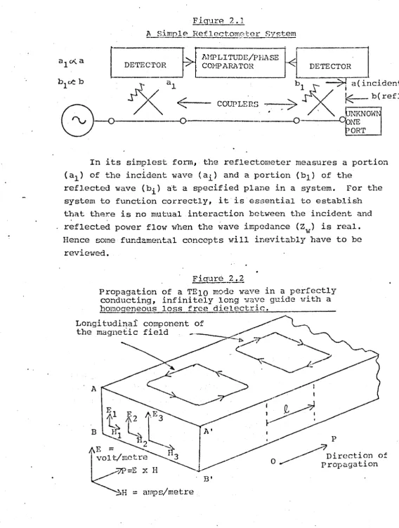
[image:41.591.4.573.42.795.2]

Figure 2.1

~~'i;i.mpl§'.:-Ref lect"o~5? .. ter ~stem

Al1PLITUDE/PHASE i

J--

J

COHPARATOR

-<E~TECTOR

b_l

><4

a( incident)

..r

~ b(refl)

COUPLERS "

"" /"" ,

G~KNOW~

--0 Op1\TE

t~_..;:.O ... R..;:.T _ _ 1

,---0,---In its simplest fona, the reflectometer measures a portion ( a₁) of the inciden"t wave (ai) and a portion (bl) of the

reflected wave (b_i ) a"t a specified plane in a syst(~m. For the system to function correctly, i t is es::-mntial to establish thai~ there is no mutual interaction bet.ween the incident and

.

"

reflected power flow w"hen the ~vave impedance (Zw) is real. Hence some fundamental concepts ,vill inevitably have to be

reviewed.

Propagation conducting, homogeneous

F i 9.1!r? __

?...:1.

of a TEIO mode wave in a perfectly infini tely long T;l~ve guide '-lith a loss free dielectri.~c:..!.. _ _ _ _ _ _ _ Longit.udinal

the magnetic

component of ~

field _~ ~

.. <:

~~

~~

A

. t

~2

j

E

3

B

~1 ~

l...

A' : p

t\E =

~2

Ft

~ ~

t

Ol

t/metn;'~I3

"~ ,. T-l ~l~

~"...---

0 .r"" propagation Direct.ion of 0'= .... x H

B'

27

-Consider the propaga·U.on of electro-magnetic energy (Fig 2.2) in a mediu ... rn

bound(~d

by AJ."\I BBI e.g., an infinitely long wave guide. 'The modes of ,.,ave discussed "Jill be limited to those modes which possess transverSl~ components of both electric and magnetic fields i.e., 'l'EM, TE or TH ,.,aves. since Jche longitudinal component of the field may alvays be found if the transverse components are known, there is no need.to retain the former explicitly in theory. In fact, for convenience, i t vril1 suffice to· "TOrJ~ entirely in terms of the transversa components of the electric and magnetic field strengths dc:motcd respectively by the symbol s E and H. Both these quanti·ties, E and II vary over the cross-section of the transmission system but because the spatial distribution is the same in each case (Fig 2.2), their ratios E3 = E2 = El

IT}

HZ

lTf

remains unchanged. Schelkunoff (Refs 2 .2; 2.3) recogni sed "t:his important generalization and introduced the concept of wave impedance (Zw) which is the ratio of these field

strengths so that at a given point along' the guide, '-le have in general:

Zw

=

t l -E _{• • • • •} 2.1

where _Zw

=

impedance 1.n

.

ohms· E

=

volts per metre

H

.-

amperes per metre.

When the wave guide is not infinitely long or perfectly' terminated, then the total transverse electric field (E) at any point will consist of incident and reflected parts. Each of these parts must, of course, be compounded of the transverse electric field 'components of all waves travelling in the

appropriate direction. The same arguemetl:. may be applied to the r.!agnetic field (H)

equations belovl apply,

E

II

at a

.

~. e. ,

=

=

given

E+ ₊

H+

₊

point. Hence t.he two

E _{• • • • •} 2.2

wherG the plus ~mperscript denotes an incident ,,,ave (direction OP in Fig 2.2) and the minus superscript denotes a reflected wave (direction PO in Fig 2.2). For this case, the iolave impedance (Zw) is then. defined as:

Zw :::: E+

H-F

_{• ••••} 2.1(a)

or

Ziv :::: -E

H-

_{• • • • •} 2.1(b)

substit.ution of .equations 2.1(a) and 2.1(b) into equation 2.3 will ~-8sul t i n :

H

• • • • • 2.4

If the symbols

€

and X are used to represent the

instantan8ou's values of the complex quanti ties E and H for a sinusoidal time variation, then:

Re

Ee.~"~

Re He

iswi:- ,

and writing equ.ations 2.2, 2.3 and 2.4 in il1stantaneous values will result in:

e

::::

s+

₊

E.

-

_{• • • • •}

g,

_{=: ~} +

₊

'lIt-_.~

_•

_{• • •}

_•

'{

=

£+

e:.:

Zw Z\f _{• ••••}

2.2 ( a)

2.3(a)

2.4{a)

The instantaneous pO\Ver. flux or poynting Vector, p." is given by

R

=

E x H. As "He have defined

E

and?( as the

transverse components, w'hich are at right angles, then P ::::

E.l}i

,\ .... here P is in the longintudinal direction so that:

P :::: _\.~"-(r+ _ _ - __ C:: .. .- -)

p

or

P

P

v7hi~h loS

.

the desired

=

= E+

=

p+

result.

- 29

-J.+ ₁

P

(f~-) 2

Zvl

<c.-

H

-• • • • •

The reflection coefficient ( r ) is defined as the complex r.<?-ot.:to of the reflected to 0 incident wave at any

specified point along the ~xis of propagation (Fig ~l).

2.5

On the basis of this definition, it. follows that there are two alternative ratios which can be used, because the coefficient may be expressed either in terms of the electric or mclgnetic field. The former definition yields:

E-E+ _{• • • • •} 2.6

"There

rc: =

.. Electric Reflection Coefficient and as before E+

-

Incident Electric Field

E-

₌

_{Reflected Electric Field.}

The latter definition yields:

·

,

. . .

2.7

where Magnetic Reflection Coefficient and as before Irlcident Nagnet.ic Field

Reflected Magnetic Field

Ei ther of the defini t:iOl1S of 2.6 or 2.7 may be used. lImvever, as it is more convc~nient t.o measure the electric

</. fielct the definition of 2.6 will b(~ used throughout this

assumed to be with respect to the electric field unless other-\d se sta ted.

At this stage, i t ¥Jould be best to refer to Fig 2.2 once

, + , " ,

agal.n. If Eo l.S the l.ncldent wave at 0, then at any pOl.nt P, distant

"t"

to the right of 0 in the direction of

propa.gation, t.he elecmc field Ep + is given by:

E +

p :: E o +

e

-pl where the propagation constant (1))=. 0{ -+

JP

• • • • •

0{ :: the attenuation constz.nt (Nepers/Hetres)

f3

=

the phase constant (Radians/Hetre).

-2.8

and and

c!' ' I 1

... ,l.ml. a.r y if E

0 is the value of the reflected "rave at

0, then E

-

at the point P is given by: p

E

=

_Eo

_e

+pl

2.9

p _{• • • • •}

The nomencla·ture "incident" . ~nd "reflected" assumes the ,\-rave source to be somewhere to the left of "0" and the point

of reflection some\vhere to the' right of P. Equation 2.8 is merely a mathematical statement of the well-known fact that

-~t

'

the field at P~ suffers attenuation by a factor

e

and lags

pi!.

radians' on the field at 0 for an incident '\-rave. Equation

2.9 is

merely

a

mathematical statement

of the

same? argument

for a reflected wave.

Similarly for t.be magnetic field, ,\"e have:

II

+

p

II

P

=

=

HO+

e

-pI

p -

e+

p1

"0

• • • • • 2.10

• • • • • 2.11

. 31

-point Os thus:

E _p

=

E -}-

e -

-pl

₊

E +pl

0 ₀

e

_{• • • • • 2.12}

11 _p = _Ho +

_e

-pI + _Ho

-

e

+pl

·

_.

.

_{. .}

2.13

-Defining

r

₌ E 0

E+

0 _{• •}

• • • 2.14

.~

H

-and =

-2-Ho+

• • • • • 2.15 then from equations 2.l(a) and 2.1(b),r

=-~

·

.

.

_.,

.

_2.16

Division of equation 2.12 by 2.13 and using the substitutions of 2.14, 2.15 and 2.16 gives:

E

=

E+

--R 0

H

P H~ · 0 • • • • •

If Schellcunoff' s definition in equation 2.1 is sub-stituted:

z'-

1

+

r

e.

+2pl

r

e,.+2pl • • • • •

2.17

2.18

The above stat.ement is general. Z t.. signifies the vrave impedance at any arbitrary point point P, situated a distance

liD.."

from the reference point 0 (Fig 2.2) Zw is the

character-istic wave impedance of the line.

If constraints are placed on the line length to ma]ce

t

= 0, equation 2.18 reduces t.o another 'veIl-known expression:

Z _L-

=

...]L _ _ _ _ Z (I

+

r )

_

(1 -

r )

_{• • • • •} 2.18(a)

r

=

z

'-Z L

• • • It • 2.19

Equation 2. 19 is the very important relationship ,-rhich forms the basis of these measurements. I t follmvs that if the characteristic impedance Z can be accurately defined

w

then measuring the complex quantityr; will allo", Z L. to be evaluated.

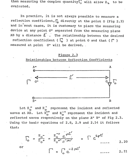
In practice, i t is not always possible to measure a reflection coefficient,ro directly at the point 0 (Fig 2.3)

.

.

,

.

'and J.ll most cases, J.t J.S customary to place the measuring device at any point

ou

separat.ed from the measuring plane

AB by a distance

i'

' e ' The relationship between the desired reflection coefficient (~ ) at point 0 and tbat (

r )

measured at point 0" will be derived.

Figure 2.3

Relationship's bet-~lcen Reflection Coefficients

A" A

G

4

t

t>

r

0" 0 _,.

1:;

"

o~--··---B"

B

LGt E + and

E-o represent the incident and reflected o

,,,aves at AB. Let E+';' and E -'I represent the incident and

o 0

reflected '\~~aves respectively on the plane A" B" of Fig 2.3. Using the basic equations of 2.8, 2.9 and 2.14 i t follmvs that:

=

or

E -...JL

E +

a

=

," ~

"'1, ~

Eo

e...

.

E +" -f~

o

e

r

=

., .. , I

I'

-~.~

<:>

e

=

• • • • • • • • • •

2.20

[image:47.586.54.546.179.792.2]

- 33

-Being complex, the reflection coefficients

.r

and ~ may be written as

jr

jeS

f

and

I~

\c!t.:.

respec·t.ively ,{here

1)

and

CPo

represent the angle in radians. substitution in 2.21 results in:

I I

r

e.

.;

'r .l

~ \~

Ie

; ,/. 10

e

-.z

r

~ =

l .

r~

I

e

t

~.Ju

I

e

_2,.0(

fi.!.

i

d .< _I

3e:

I

rll9'>=

[i

~

I

e.-

0at]

e

j. (¢o

-2.1'12:)

• • • • •

From which i t is easily seen that the modulus of the measured reflection coefficient i's att:enuat.ed by a factor

n~ .

2

ex

x... from the,true modulus, Vlhi1st the angle of the

2.22

measured reflection coefficient is modified by t.he difference 2

I~

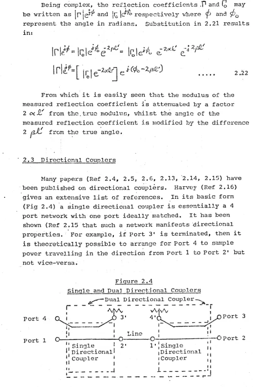
from the true angle •

. 2.3 Di.rectiona1 Couplers

:Hany papers (Ref 2.4, 2.5, 2.6, 2.13, '2.14, 2.15) have . been published on directional co~p1ers. Harvey (Ref 2.16)

,

gives an extensive list of references. In its basic form (Fig 2.4) 'a single directional coupler is essentially a 4 port network with one port ideally matched. It has been

shown (Ref 2.15 that such a net'\vork manifests 'directiona1 properties. For example, if Port 3' is terminated, then i t

is theoretically possible to arrange

for

Port

4

t.o sample power travelling in the direction from Port 1 to Port 2' but not vice-versa.

port 4

[image:48.583.48.549.52.818.2]

port 1

Figure 2.4

Sinqle alld Dual Directional Couplers u---Dual Directional Coupler--;".

:- - -

--~-"

- - -

'A~1'v

- - - -:

3

0... ',_ ,_ _ _ _ _

_I 3' 4' _ _ _ _ _ _ ..1 J

P

Port

TC=--_.

I

--~

I I I '.

" T ' I I

I I .u1ne I . - 0

o

0- 0 . ~ Port 2

I i . J" I • i ," i I

. Slng .. e 2' 1 I 5

₇

ng1G. Ii

I'Direct.ionall I Dl.rectl.onal 'i

II Coupler I I Coupler 'I

t I ' 1 ,

II

1

II

, __ ._ --I ----.---~II

,...----;:0---coup1 ers are required, on(~ to sample the inciden·t "Jave and the other to sampl(:! the reflected wave. The use of . two

separate couplers joined by a connecting line is undesirable because of mis-matches between the units. Difficulty is experienced with attaining amplitude and phase tracking. To alleviate these undesirable effects, manufacturers tend to offer dual directional couplers units for 1vhich claims arc made that the internal couplers are matched for ampli-tude and phase.

A dual direc·tional coupler may be analysed as a four port netvrorlc (Fig 2.4) vli th the general scattering matrix of eq~ation 2.23.

Samples t-i <11_ Incident POIver

Source

- 35

--. Fiqnre 2 --.4(

al

Signc.l Flow G.r-aph of a Dual _ _ ..:::D:;...:irect:is:mal G.oupler

C = Desired coupling paths CD

=

Back coupling paths

Load

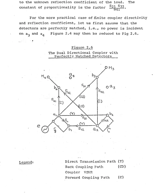
Tbe F0;l'lvard ~.9uRling Patq (C) I is' the desired signal path

from one por~ to another •. These are 8

41 for port 1 to port 4 and _{8 32} for port 2 to 3.

!.11g--1}_~.£.1~ CQllPlj..ng P_~IJ:}lf1 (CD ) I are the undesired signal paths

to a particular port. The paths are 542 for por·t. 4 and 531

for port 3.

!

Incident POvler to Port 1

Incident PO·v:er to Port 4

·

. .

.

.

2.24

Direct:i vi ty Fact.or (DIE1=10 log

r

POv:er to Port 4 POi'lCr to Port 3

·

.

.

. .

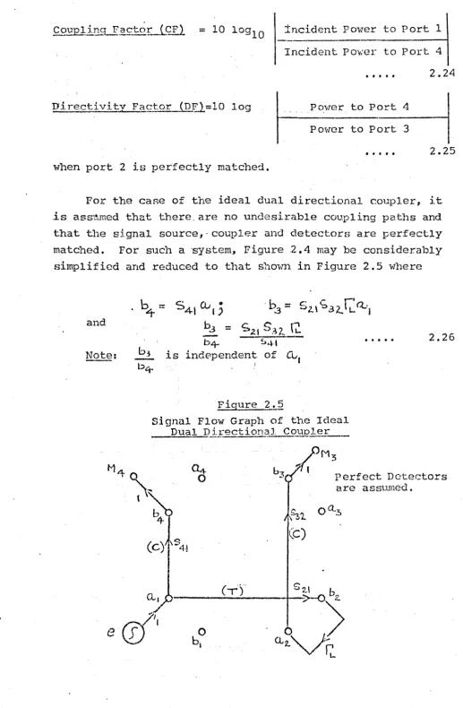
2.25 w'hen port 2 is perfectly matched.

For the case of the ideal dual directional coupler, i t

is ass1.~med that there, are no undesirable coupling pcl.ths and that the signal source,' coupler and detectors are perfectly matched. For such a 'system, Figure 2.4 may be considerably

simplified and reduced to that s1'1own in Figure 2.5 "there

and

.b

₄

:"::

S41Q;,)

'b.3=

S2.\S32..~Q..1

b3 ₌ £.21

S.~?. ~

b4- S4'

[image:51.585.35.552.30.820.2]

is independent. of CV 1

Figure 2.~

Signal Flow Graph of the Ideal Dual Directional Coupler

_-",-",-,;;~..:.o-_ _ _ • • . - - - _ _ _ _ _

·

. .

. .

2.26

Perfect Detectors are assumed.