Analytical model of the crossed wire particle velocity sensor
Twan Spil s1227718 Bachelor assignment committee
prof.dr.ir. GJM Krijnen prof.dr.ir. A. de Boer
ir. O. Pjetri
Abstract
Contents
1 Introduction 2
2 Analytical model 4
2.1 Static thermal profile . . . 4
2.1.1 One wire . . . 4
2.1.2 Two wires . . . 7
2.2 Thermal heat profile with Finite width . . . 8
2.2.1 One wire . . . 8
2.2.2 Heat loss through the wire . . . 10
2.2.3 Two wires . . . 11
2.2.4 Comparison with simulation . . . 11
2.3 Static disturbance thermal profile . . . 12
2.3.1 Wire perpendicular to air flow . . . 12
2.3.2 Wire parallel to airflow . . . 13
2.4 Dynamic disturbance thermal profile . . . 15
2.4.1 Flow perpendicular to the wire . . . 15
2.4.2 Flow parallel to the wire . . . 16
2.5 Sensitivity . . . 16
2.5.1 Comparison with measurements . . . 17
3 Reduced model 19 3.1 Thermal profile . . . 19
3.2 Perturbation flow parallel . . . 20
3.3 Perturbation flow perpendicular . . . 21
4 Exploration parameter space 22 4.1 Square chiply=lx. . . 22
4.2 Width of the wire . . . 23
5 Discussion and Conclusion 24 5.1 Discussion . . . 24
5.2 Recommendations . . . 24
Chapter 1
Introduction
[image:4.595.152.449.405.493.2]The subject of this Bachelor Assignment is acoustic particle velocity sensing based on thermal sen-sors. There are various configurations for these sensors, most of them relying on either two heated wires, or one heated wire and two measurement wires [3, 4]. These sensors work as follows, a current is put through the heating wire(s) and power is dissipated as heat. The heat will cause a thermal pro-file over the sensor. When an acoustic particle velocity, aka a sound wave, travels over the sensor, the thermal profile will be disturbed. This flow disturbance leads to a temperature difference between the measuring wires that causes a change in resistance which is then measured by measuring the voltage over the wires when an equal current flows through the wires. For the configurations with either two heated wires, or one heated wire and two measurement wires an analytical model has al-ready been developed.
Figure 1.1: The configuration with one heater wire and two sensor wires for which an analytical model already has been developed [3]
In this work the focus is on a so called crossed wire sensor geometry. The crossed wire sensor [2] de-viates from previous configurations, because now the wires are both heaters and sense the resistance variations and more importantly, the temperature variations are caused by flows parallel to the wires and measured along the longitudinal direction, this is also illustrated in figure 1.2 (c). In the crossed wire sensor, the wires are heated by forcing a current through the wires this is illustrated in figure 1.2 (b). In a static situation when there is no particle velocity over the sensor, the thermal profile will be symmetric and the resistances of the wires will be equal. Due to an equal current being forced over the wires, the voltages will also be equal and the difference of the voltages between the ends of the wire will be zero. When a sound wave travels over the sensor, for example over R2 and R5, the resis-tance changes differently for R2 then it does for R5, and the difference between the voltageV1+−V1−
will be non-zero.
for the thermal profile when there is a static flow disturbance and finally I made a model for the ther-mal profile with dynamic flow disturbances. From these flow disturbances it is possible to predict the sensitivity. The model is compared with measurements to assess their predictive quality.
[image:5.595.85.508.132.280.2](a) (b) (c)
Figure 1.2: (a) Image from a top view of the crossed wire 2D particle velocity sensor [2] (b) A schematic of how the forced currents flow through the wires of the sensor (c) A drawing of how the flow affects the temperature profile over the wires (resistors)
ly
lx
2L x
y
air flow
y x
[image:5.595.88.509.354.491.2]Chapter 2
Analytical model
2.1 Static thermal profile
2.1.1 One wire
To gather some insight I will start with a somewhat different geometry, which can be seen in figure 2.1. To make a analytical model for the thermal profile we start with the heat equation.
−∇(k∇T)=Q (2.1)
Wherekis the gas thermal conductivity, which has a dependence on T but for the sake of simplicity we assume it to be negligible.Qis the heat quantity produced by the wire. It is only non zero on the position where the wire is located and is distributed evenly along the wire that it can be written as.
Q=P
lyδ(x)δ(z) (2.2)
Where P is the power dissipated by the wires as heat andly the length of the wire. The positional dependence is taken into account with the delta functions, this can be done because the length of the wire is much bigger then the width or the thickness. Later on in this report the finite thickness is also taken into consideration. Putting the expression forQ into (2.1) together with the assumption thatkdoes not depend on temperature nor position, results in a linear partial differential equation.
−k µ ∂2
∂x2+
∂2
∂y2+
∂2
∂z2 
T(x,y,z)=Q (2.3)
z y
ly
y x
[image:6.595.157.460.521.706.2]lx
We can solve this equation using eigenfunction expansion [1], we start with the homogeneous partial differential equation and solve for y with separation of variables. For the boundary condition we use thatT(x,±l2y,z)=0, where the ambient temperature is taken zero. The walls on±l2y in figure 2.1 extent to infinity.
−k µ ∂2
∂x2+
∂2
∂y2+
∂2
∂z2 
T(x,y,z)=0 (2.4)
T(x,y,z)=T x(x,z)Y(y) (2.5)
−
³∂2
∂x2+ ∂ 2
∂z2
´ T x
T x =
∂2
∂y2Y
Y (2.6)
∂2
∂y2Y
Y = −λ (2.7)
∂2
∂y2Y +λY =0 (2.8)
Y(±ly
2)=0 (2.9)
Y(y)=cos
µ2λ
ny
l y 
(2.10)
λn=π
2(2n+1) (2.11)
T(x,y,z)=
∞
X
n=0
Tn(x,z) cos
µ2λ
ny
ly 
(2.12)
Filling this into (2.3) results in
∞
X
n=0 ·µ ∂2
∂x2+
∂2
∂z2 
Tn−
µ2λ
n ly ¶2 Tn ¸ cos
µ2λ
ny
ly 
= − P
lykδ(x)δ(z) (2.13)
Due to orthogonality
µ ∂2
∂x2+
∂2
∂z2 
Tn−
µ2λ
n
ly ¶2
Tn=
2
ly Z ly
2
−l2y
− P
lykδ(x)δ(z) cos µ2λ
ny
ly 
dy (2.14)
= − P
lykδ(x)δ(z)
2 sin(λn)
λn
(2.15)
= −2(−1)
n
λn
P lykδ
(x)δ(z) (2.16)
Using the Fourier transform
ˆ
Tn(kx,kz)=
Z ∞
−∞
Z ∞
−∞
Tn(x,z)e−i(kxx+kzz)dxdz (2.17)
to (2.16)
¡
−kx2+ −kz2¢ ˆ Tn−
µ2λ
n
ly 
ˆ
Tn= −
2(−1)n
λn
P
lyk (2.18)
ˆ
Tn=
2(−1)n λn
P ly
kx2+ky2+³2λn
ly
Figure 2.2: 3D plot of the temperature profile (2.22) depending on x and y withz=1µm
The Fourier transform of a second kind modified Bessel function is
F[K0(ar)]=
1 2π
1
k2+a2 (2.20)
If we assume for our solution that the frequency is radialk=
q
kx2+kz2then we can take the inverse
transform to get
Tn(x,z)=
2(−1)n
λn
P
2πlykK0 Ã
2λn
p
x2+z2 ly
!
(2.21)
Filling everything back together results in
T(x,y,z)=
∞
X
n=0
2(−1)n
λn
P
2πlykK0 Ã
2λn
p
x2+z2 ly
!
cos
µ2λ
ny
ly 
(2.22)
A plot of this solution can be seen in figure 2.2. The parameters used for all the graphs in this chapter can be found in the table below.
ly lx 2L k P v
900µm 900µm 2µm 0.0386 W K−1m 26 mW 4.4
2.1.2 Two wires
Due to linearity of the heat equation it is possible to just add up the two thermal profiles for the two wires which are the same but with reversed x and y. Resulting in
T(x,y,z)=
∞
X
n=0 "
2(−1)n
λn
P
2πlyk K0
Ã
2λn
p
x2+z2 ly
!
cos
µ2λ
ny
ly 
+
2(−1)n
λn
P
2πlxk K0
Ã
2λn
p y2+z2 lx
!
cos
µ2λ
nx
lx ¶#
(2.23)
This equation is plotted in figure 2.3
Figure 2.3: 3D plot of the temperature against x and y of the equation with two wires (2.23) with
2.2 Thermal heat profile with Finite width
2.2.1 One wire
ly
lx
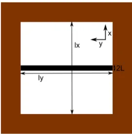
[image:10.595.229.365.125.263.2]2L x y
Figure 2.4: Geometry used for developing the analytical model for the thermal profile with a finite width
Starting from the same heat equation
−∇(k∇T)=Q (2.24)
But now we take into account a finite width for the wires. The total width is 2L
Q= P
2LlyF(x)δ(z) (2.25)
F(x)=
½
1 |x| <L
0 otherwise
¾
(2.26)
Assuming thatkis constant
µ ∂2
∂x2+
∂2
∂y2+
∂2
∂z2 
T= − P
2Lkly
F(x)δ(z) (2.27)
The boundary conditions
T(±lx
2,y,z)=0 (2.28)
T(x,±ly
2,z)=0 (2.29)
T(x,y,±∞)=0 (2.30)
using the method of separation of variables.
µ ∂2
∂x2+
∂2
∂y2+
∂2
∂z2 
T=0 (2.31)
T(x,y,z)=Θ(x,y)Z(z) (2.32)
³∂2
∂x2+ ∂ 2
∂y2
´ Θ(x,y)
Θ(x,y) =
∂2
∂z2Z(z)
Z(z) (2.33)
³
∂2
∂x2+ ∂ 2
∂y2
´ Θ(x,y)
Θ(x,y) = −λ (2.34)
Θ(x,y)=cos
µ2λ
my
ly 
cos
µ2λ
nx
lx 
(2.35)
Withλn= pi2(2n+1) andλm= pi2 (2m+1) such that the temperature is zero at the boundaries± ly
2
and±lx
2.
T(x,y,z)=
∞
X
n=0
∞
X
m=0
Tnm(z) cos
µ
2λmy
ly 
cos
µ
2λnx
lx 
(2.36)
Now filling this back into the heat equation we get
∞
X
n=0
∞
X
m=0 · ∂2
∂z2Tnm− µµ2λ
n
lx ¶2
+
µ2λ
m
ly ¶2
Tnm
¸
cos
µ2λ
my
ly 
cos
µ2λ
nx
lx 
(2.37)
= − P
2Lkly
F(x)δ(z)
Due to orthogonality
µ ∂2
∂z2− µ2λ
n
lx ¶2
−
µ2λ
m
ly ¶2
Tnm (2.38)
= −2
ly
2
lx Z l2x
−lx 2
Z
ly 2
−l2y−
P
2Llyk
F(x)δ(z) cos
µ2λ
my
ly 
cos
µ2λ
nx
lx 
dydx (2.39)
= −(−1)
mP
λmLlykδ
(z)
Z L
−Lcos
µ2λ
nx
lx 
dx (2.40)
= −2(−1)
m
λmλn
P Llyksin
µ2λ
nL
lx 
Figure 2.5: 3D plot of the temperature profile (2.47) depending on x and y withz=0
Using the Fourier Transform
ˆ
Tnm(kz)=
Z ∞
−∞
Tnme−i kzzdz (2.42)
µ k2z+
µ2λ
n
lx ¶2
+
µ2λ
m
ly ¶2
ˆ
Tnm=
2(−1)m
λmλn
P Llyk
sin
µ2λ
nL
lx 
(2.43)
ˆ
Tnm=
2(−1)m λmλn
P Llyksin
³2λ
nL
lx
´
kz2+ r
³2λ
n
lx
´2
+³2λm
ly
´22
(2.44)
F−1µ 2a k2
z+a2 
=e
−a|x|
2π (2.45)
Tnm=
(−1)m
λmλn
P Llyksin
³2λ
nL
lx
´
r ³2λ
n
lx
´2
+
³2λ
m ly ´2 exp(− s µ
2λn
lx ¶2
+
µ
2λm
ly ¶2
|z|) (2.46)
Putting it all together, resulting in the solution
T(x,y,z)=
∞
X
n=0
∞
X
m=0
(−1)m
λmλnσnm
P Llyksin
µ2λ
nL
lx 
exp(−σnm|z|) cos
µ2λ
my
ly 
cos
µ2λ
nx
lx 
(2.47)
σnm=
s µ2λ
n
lx ¶2
+
µ2λ
m
ly ¶2
(2.48)
A plot of this can be seen in Figure 2.5.
2.2.2 Heat loss through the wire
Figure 2.6: 3D plot of the temperature profile with two wires (2.50) depending on x and y withz=0
walls. The heat power dissipated trough the beam ends∆P, is the product of the heat flux through the wire ends and the area of the wire cross section.
∆P=2kw∂T
∂yy=ly 2
h2L (2.49)
Working this out and filling it in withkw=18.5 W K−1m andh=0.1µm results in ∆PP =0.0263. So
less then 3% of power is dissipated on the wire end, this means that the assumption that only a small portion of the power is dissipated at the wire ends.
2.2.3 Two wires
Using the thermal profile we got and combining it results in the following equation.
T(x,y,z)=
∞
X
n,m=0
(−1)m
λmλnσnm
P Llyksin
µ2λ
nL
lx 
exp (−σnm|z|) cos
µ2λ
my
ly 
cos
µ2λ
nx
lx 
(2.50)
+
∞
X
n,m=0
(−1)m
λmλnσnm
P Llxksin
µ2λ
nL
ly 
exp (−σnm|z|) cos
µ2λ
mx
lx 
cos
µ2λ
ny
ly 
The plot can be seen in Figure 2.6.
2.2.4 Comparison with simulation
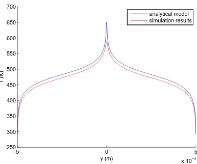
−5 0 5 x 10⁻⁴ 250
300 350 400 450 500 550 600 650 700
y (m)
T (K)
[image:14.595.197.390.78.239.2]analytical model simulation results
Figure 2.7: A plot of the temperature profile of the analytical model and temperature profile from the simulation against y withx,z=0
2.3 Static disturbance thermal profile
2.3.1 Wire perpendicular to air flow
Due to the air flow there are two more terms in the heat equation.
ρcp
µ∂
∂tT+v· ∇T 
− ∇(k∇T)=Q (2.51)
Where v is the gas velocity,ρandcp the density and heat capacity of the gas, the heat capacity and
density of the wires aren’t taken into account in this equation, this is done for the sake of simplicity. The time differential of T is zero because T is assumed to have only a static disturbance, thus no dependence on time.
The convective term in equation (2.51) can be treated as a perturbation because the diffusion velocity is large in comparison with the forced convection caused by the particle velocity. Let’s look at how long it takes for a particle to travel over the length of the sensorlx: due to diffusion this time will
belx2/D withD =k/ρcp≈1.9×10−5m2s−1, due to forced convection this time will belx/v. If we
compare these times with each other
v D/lx¿
1 (2.52)
Because the diffusion velocity D/lx≈0.02 m s−1 is large in comparison with v = 4.4×10⁻³m s−1
(which corresponds to a very high acoustic pressure of 100 dB). Therefore we can consider the tem-perature asT+δT whereT is the temperature in non-flowing air that was already found and δT
the perturbation caused by the flowing air. We will solve the case for air flowing in one direction v=(vx, 0, 0).
∇2δT =vx
D
∂
∂xT (2.53)
∂ ∂xT=
∞
X
n=0
∞
X
m=0
−Cnm×exp (−σnm|z|) cos
µ2λ
my
ly 
sin
µ2λ
nx
lx 
(2.54)
Cnm=
2(−1)m
λmσnm
P Llylxk
sin
µ2λ
nL
lx 
(2.55)
∇2δT=
∞
X X∞
−Cnm
vx
D exp(−σnm|z|) cos µ2λ
my
ly 
sin
µ2λ
nx
lx 
To solve this equation one should again use the eigenfunction expansion, but this time a cosine for the x-direction will not work, because the integral of a sine and cosine over the length of the wire results in zero. Thus we use a sine that satisfies the boundary conditions.
δT=
∞
X
i=0
∞
X
j=1
δTi j(z) cos
µ2λ
i
ly y
sin
µ2πj lx
x 
(2.57)
Substituting this into (2.56) and again orthogonalising the various terms yields
µ ∂2
∂z2− µ2λ
i
ly ¶2
−
µ2πj lx
¶2
δTi j(z)=
∞
X
n,m=0 h
−Cnm
vx
D exp(−σnm|z|)×
2
ly Z ly
2
−l2y cos
µ2λ
my
ly 
cos
µ2λ
iy
ly 
dy2 lx
Z lx
2
−l2x sin
µ2λ
nx
lx 
sin
µ2πj x lx ¶ dx # (2.58) 2 ly Z ly 2
−l2y cos
µ2λ
my
ly 
cos
µ2λ
iy
ly 
dy=
½
1 m=i
0 m6=i ¾
(2.59)
2
lx Z l2x
−lx 2
sin
µ2λ
nx
lx 
sin
µ2πj x lx
dx= −2πj(−1)
n+j
π2j2−λ2
n
(2.60)
µ∂2
∂z2− µ2λ
m
ly ¶2
−
µ2πj lx
¶2
δTj m(z)=
∞
X
n=0 Cnm
vx
D
2πj(−1)n+j
π2j2−λ2
n
exp(−σnm|z|) (2.61)
Now we assume a solution for the ordinary differential equation (2.61),δTj m(z)=Aj mexp(−σnm|z|).
∂2
∂z2Aj mexp(−σnm|z|)=Aj mσ 2
nmsign(z)2exp(−σnm|z|)=Aj mσ2nmexp(−σnm|z|) (2.62)
µ
σ2
nm−
µ2λ
m
ly ¶2
−
µ2πj lx
¶2¶ Aj m=
∞
X
n=0 Cnm
vx
D
2πj(−1)n+j
π2j2−λ2
n
(2.63)
µµ2λ
n
lx ¶2
−
µ2πj lx
¶2¶ Aj m=
∞
X
n=0 Cnm
vx
D
2πj(−1)n+j
π2j2−λ2
n
(2.64)
Aj m=
∞
X
n=0
−Cnmlx2 vx
D
πj(−1)n+j
2(π2j2−λ2
n)2
(2.65)
δT=
∞
X
m,n=0
∞
X
j=1
−(−1)
m+n+j
λmσnm
Plx Llyksin
µ2λ
nL lx ¶v x D πj γ2 n j
exp(−σnm|z|) cos
µ2λ
i
ly y 
sin
µ2πj lx x
(2.66)
withγn j=π2j2−λ2na plot of this perturbation and the effect on the temperature profile can be seen
in figure 2.8.
2.3.2 Wire parallel to airflow
We repeat what we did in the previous section, only now what is different is that we differentiate the temperature profile with respect tox, resulting in the following partial differential equation:
∇2δT=
∞
X
n,m=0
−Cnmexp(−σnm|z|) sin
µ2λ
mx
lx 
cos
µ2λ
ny
ly 
(2.67)
Cnm=
2(−1)m
λnσnm
P Ll2 xk
sin
µ2λ
nL
ly 
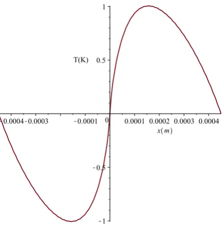
Figure 2.8: Plot of the temperature perturbation (2.72) for a flow perpendicular to the wire depending on x, withy,z=0
We solve this equation using eigenfunction expansion in the same way as we did it with the airflow perpendicular to the wire. This results in an ordinary differential equation.
µ ∂2
∂z2− µ2λ
n
ly ¶2
−
µ2πj lx
¶2
δTj(z)=
∞
X
m=0 Cnm
vx
D
2πj(−1)m+j
π2j2−λ2
m
exp(−σnm|z|) (2.69)
This equation is easily solved by assuming a solutionTj(z)=Aexp(−σnm|z|)
µ
σ2
nm−
µ2λ
n
ly ¶2
−
µ2πj lx
¶2¶ A=
∞
X
m=0 Cnm
vx
D
2πj(−1)m+j
π2j2−λ2
m
(2.70)
A=
∞
X
m=0
−Cnmlx2 vx
D
πj(−1)m+j 2(π2j2−λ2
m)2
(2.71)
Combining everything the solution of the perturbation of the temperature is found:
δT=
∞
X
n,m=0
∞
X
j=1
− (−1)
j
λnσnm
P Lksin
µ2λ
nL
ly ¶v
x
D
πj
γ2
m j
exp(−σnm|z|) cos
µ2λ
n
ly y 
sin
µ2πj lx x
(2.72)
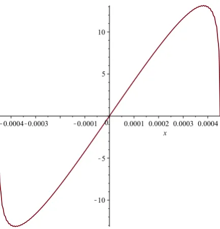
withγm j=π2j2−λ2ma plot of this perturbation affecting the temperature profile can be seen in figure
Figure 2.9: Plot of the temperature perturbation (2.66) due to a flow parallel to the wire depending on x, withy,z=0
2.4 Dynamic disturbance thermal profile
2.4.1 Flow perpendicular to the wire
Using the same heat equation as in the previous section, with the same assumptions,
ρcp
µ∂
∂tT+v∇T 
− ∇(k∇T)=Q (2.73)
but now we don’t assume the time dependence to be zero. The sensor deals with sound waves, which are acoustic, so we assume the incoming particle velocity to bev=v0exp(i2πf t). Due to this being the only time depending term in the heat equation, we can also assume the solution to be of the form
δT(x,y,z,t)=δT(x,y,z) exp(i2πf t). Using that we only have an x component of the particle velocity v=(v, 0, 0) we get for the convective termv∇T=v∂∂xT.
i2πf
D δT− ∇ 2δT
= −v0
D
∂
∂xT (2.74)
This is almost the same equation as we had in the previous section and we can solve it in the same way using eigenfunction expansion. First we begin with constructing a solution for the perturbation of the temperature for the wire perpendicular to the x direction.
µ
−i2πf
D +
∂2
∂z2− µ2λ
m
ly ¶2
−
µ2πj lx
¶2
δTj m(z)=
∞
X
n=0 Cnm
v0 D
2πj(−1)n+j
π2j2−λ2
n
exp(−σnm|z|) (2.75)
Cnm=
2(−1)m
λmσnm
P Llylxk
sin
µ2λ
nL
lx 
(2.76)
The above equation can be solved by assumingδTj m(z)=Aj mexp(−σnm|z|).
Aj m=
∞
X
n=0 Cnm
v0 D
2πj(−1)n+j
¡
π2j2−λ2
n
¢ Kn j
(2.78)
Kn j =
µ2λ
n
lx ¶2
−
µ2πj lx
¶2
−i2πf
D (2.79)
Putting everything back together gives the temperature perturbation for a flow perpendicular to the wire.
δT(x,y,z,t)=
∞
X
n,m=0
∞
X
j=1
2(−1)m
λmσnm
P Llylxksin
µ2λ
nL
lx ¶v
0 D
2πj(−1)n+j
¡
π2j2−λ2
n
¢ Kn j
(2.80)
×cos
µ2λ
m
ly y 
sin
µ2πj lx x
exp(−σnm|z|) exp(i2πf t)
2.4.2 Flow parallel to the wire
For the flow parallel to the wire we can do the same as we did above only now we have a different∂∂xT
term. After eigenfunction expansion that leads to the following equation.
µ
−i2πf
D +
∂2
∂z2− µ2λ
n
ly ¶2
−
µ2πj lx
¶2
δTj n(z)=
∞
X
m=0 Cnm
v0 D
2πj(−1)m+j
π2j2−λ2
m
exp(−σnm|z|) (2.81)
Cnm=
2(−1)m
λnσnm
P Ll2xk
sin
µ2λ
nL
ly 
(2.82)
Using thatδTj n=Aj nexp(−σnm|z|) results in the following equation.
Aj n=
∞
X
m=0 Cnm
v0 D
2πj(−1)m+j
¡
π2j2−λ2
m
¢ Km j
(2.83)
Km j=
µ2λ
m
lx ¶2
−
µ2πj lx
¶2
−i2πf
D (2.84)
Combining everything results in the temperature perturbation for the flow parallel to the wire.
δT(x,y,z,t)=
∞
X
n,m=0
∞
X
j=1
2
λnσnm
P Llx2k
sin
µ2λ
nL
ly ¶v
0 D
2πj(−1)j
¡
π2j2−λ2
m
¢ Km j
(2.85)
×cos
µ2λ
n
ly y 
sin
µ2πj lx x
exp(−σnm|z|) exp(i2πf t)
2.5 Sensitivity
To calculate the sensitivity we first calculate the average temperature of the perturbation over the wires. To calculate this average, integration over the temperature perturbation is performed over the length, width and thickness of the upper part of the wire.
1 2L
Z L
−L
cos
µ2λ
my
ly 
dy=
lysin ³2λ
my
ly
´
2Lλm
(2.86)
2Z l2x
sin
µ2πj x
dx= −((−1)
j
−1)
exp(−σnm|z|)δ(z)=1 (2.88)
Contribution from wire parallel to flow
∆T=
∞
X
n,m=0
∞
X
j=1
− 2
λnσnm
P Llx2k
sin
µ2λ
nL
ly ¶v0
D
2πj(−1)j
¡
π2j2−λ2
m
¢ Km j
(2.89)
×
lysin³2λnL
ly
´
2Lλn
((−1)j−1)
πj exp(i2πf t)
Contribution from wire perpendicular to flow
∆T =
∞
X
n,m=0
∞
X
j=1
−2(−1)
m
λmσnm
P Llylxk
sin
µ2λ
nL
lx ¶v0
D
2πj(−1)n+j
¡
π2j2−λ2
n
¢ Kn j
(2.90)
×
lysin³2λmL
ly
´
2Lλm
((−1)j−1)
πj exp(i2πf t) (2.91)
From this averaged temperature we can calculate the resistance
R=R0(1+α∆T) (2.92)
In [3] values forR0=683Ωandα=8.6×10⁻⁴K were derived.
From the resistance we can calculate the voltage difference between the two terminals. The temper-ature difference of the upper and lower part of the wire are opposite which means that the resistance is also opposite.
V2+−V2-=I(R1−R2)=2I R0α∆T (2.93)
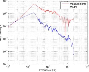
2.5.1 Comparison with measurements
101 102 103 104 105 10−4
10−3 10−2 10−1 100 101
Frequency (Hz)
Responsivity V
[image:20.595.115.469.254.537.2]Measurements Model
Chapter 3
Reduced model
In this chapter I will be looking at the possibility of reducing (decreasing the sums in an equation to an equation that consists of only a few terms) the equation for the thermal profile and it’s perturba-tions.
3.1 Thermal profile
The equation for the thermal profile is as follows
T(x,y,z)=
∞
X
n=0
∞
X
m=0
(−1)m
λmλnσnm
P Llyksin
µ2λ
nL
lx 
exp(−σnm|z|) cos
µ2λ
my
ly 
cos
µ2λ
nx
lx 
(3.1)
σnm=
s µ2λ
n
lx ¶2
+
µ2λ
m
ly ¶2
(3.2)
λm=π
2(2n+1) (3.3)
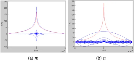
To determine if the equation could be reduced, plots were made in the following way. The sum-variable that was investigated was substituted with zero while the other sum-sum-variable(s) were summed to a hundred, this was plotted, and then it was substituted for one, etc. up to one hundred. This re-sulted in the following graphs figure 3.1 and 3.2. From these graphs you can easily see that you only need a few terms ofmto have a quite a good approximation, fornthis isn’t the case and you will need to go up to quite a large number.
[image:21.595.159.438.549.675.2](a)m (b)n
(a)m (b)n
Figure 3.2: Plots of how the values ofmandn(blue) contribute to the thermal profile (red). For the wire parallel to they-axis
3.2 Perturbation flow parallel
The equation for the temperature perturbation with a flow parallel to the wire, withγn j=π2j2−λ2n
δT(x,y,z,t)=
∞
X
n,m=0
∞
X
j=1
2
λnσnm
P Llx2k
sin
µ2λ
nL
ly ¶v0
D
2πj(−1)j
¡
π2j2−λ2
m
¢ Km j
(3.4)
×cos
µ2λ
n
ly y 
sin
µ2πj lx x
exp(−σnm|z|) exp(i2πf t)
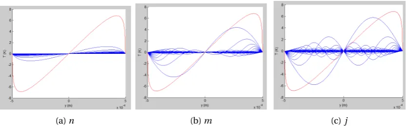
Plotting this equation in the same way we did as in the previous section we get the following graphs, figure 3.3. As can be seen, formand jyou need to sum to at least 3-5 terms. For n this is a lot more, in the range of 50-100 terms.
(a)n (b)m (c) j
[image:22.595.90.510.426.556.2]3.3 Perturbation flow perpendicular
The equation for the temperature perturbation with a flow perpendicular to the wire
δT(x,y,z,t)=
∞
X
n,m=0
∞
X
j=1
2(−1)m
λmσnm
P Llylxksin
µ2λ
nL
lx ¶v0
D
2πj(−1)n+j
¡
π2j2−λ2
n
¢ Kn j
(3.5)
×cos
µ2λ
m
ly y
sin
µ2πj lx
x 
exp(−σnm|z|) exp(i2πf t)
Plotting this equation in the same way as in the previous sections results in figure 3.4, m and j only need a few 1-3 terms to describe the perturbation, but for n some more terms 10-15 are needed.
[image:23.595.86.512.226.355.2](a)n (b)m (c) j
Chapter 4
Exploration parameter space
In this chapter I will explore how the different parameters of the micro-flown affect the sensitivity, the averaged temperature of the perturbation, over a frequency range.
4.1 Square chip
l
y=
l
xIn this section we will look at how the length of the wires affects the temperature of the perturbation, withly=lxsuch that the sensor will have the same sensitivity in both directions. From figure 4.1 you can see that a smaller length of the wires results in a higher corner frequency, but the sensitivity before this corner frequency will be somewhat smaller.
100 102 104 106 108
10−14 10−12 10−10 10−8 10−6 10−4 10−2
100 102
f (Hz) T (K) ly = 10 um
ly = 0.1 mm ly = 1 mm ly = 10 mm
(a)
10−5 10−4 10−3 10−2
101 102 103 104 105 106 107
ly (m)
Area under the curve
[image:24.595.99.493.393.559.2](b)
Figure 4.1: (a) The averaged temperature plotted as a function of frequency for various values ofly
4.2 Width of the wire
Now we will look how the average temperature of the perturbation changes as we change the width (L) of the wire. As can be seen in figure 4.2 it looks like the sensitivity only changes when the value of
Lapproaches that ofly=1×10⁻³m.
100 102 104 106 108
10−12 10−10
10−8 10−6 10−4 10−2 100
102
f (Hz)
T (K)
L = 10 nm L = 0.1 um L = 1 um L = 10 um L = 0.1 mm L = 0.5mm
(a)
10−9 10−8 10−7 10−6 10−5 10−4
102 103 104
L (m)
Area under the curve
[image:25.595.98.491.156.319.2](b)
Chapter 5
Discussion and Conclusion
5.1 Discussion
In the development of the analytical model a few simplifications and assumptions were made. The air thermal conductivity (k) was considered independent of temperature, in the temperature range the sensor operates 500 °C,k doubles, so that assumption isn’t really valid. We didn’t take into ac-count the bottom of the sensor at a negativezand we assumed the walls to be extending from the positivez. But as can be seen in figure 2.7 a simulation with the accurate geometry of the sensor has almost the same temperature profile. Unfortunately due to time constrains we were not able to measure the actual thermal profile of the sensor to compare it to the model.
The sensitivity according to the analytical model has roughly the same shape compared to the mea-surements of the sensitivity, but the analytical model shows a stronger decay with frequency than observed in the measurements. This could either be due to
• one of the assumptions made or due to incomplete incorporation of all effects, e.g. such as the heat capacity and thermal conductivity of the wires
• from a mistake in the derivation of the dynamic disturbance
• or because the wires have a thicker connection with the walls of the sensor, which leads effec-tively to a smaller wire.
These are subjects that could be examined in future work in order to further improve the model.
5.2 Recommendations
• Look more into noise
• Make a series of crossed wire flowns with varying length to validate influence of length on performance
• Validate the thermal profile by measurements
5.3 Conclusion
Bibliography
[1] Richard Haberman. Elementary applied partial differential equations. Prentice Hall Englewood Cliffs, NJ, 1983.
[2] O Pjetri, RJ Wiegerink, TSJ Lammerink, and GJM Krijnen. A crossed-wire 2-dimensional acoustic particle velocity sensor. InSensors, 2013 IEEE, pages 1–4. IEEE, 2013.
[3] VB Svetovoy and IA Winter. Model of theµ-flown microphone.Sensors and Actuators A: Physical, 86(3):171–181, 2000.
![Figure 1.1: The configuration with one heater wire and two sensor wires for which an analyticalmodel already has been developed [3]](https://thumb-us.123doks.com/thumbv2/123dok_us/9896909.490985/4.595.152.449.405.493/figure-conguration-heater-wire-sensor-wires-analyticalmodel-developed.webp)
![Figure 1.2: (a) Image from a top view of the crossed wire 2D particle velocity sensor [2] (b) A schematicof how the forced currents flow through the wires of the sensor (c) A drawing of how the flow affectsthe temperature profile over the wires (resistors)](https://thumb-us.123doks.com/thumbv2/123dok_us/9896909.490985/5.595.88.509.354.491/particle-velocity-schematicof-currents-affectsthe-temperature-prole-resistors.webp)