Real time operating systems, with emphasis on the man/machine interface

WITH EMPHASIS ON THE MAN/MACHINE INTERFACE

A THESIS PRESENTED FOR THE DEGREE OF DOCTOR OF PHILOSOPHY IN CHEMICAL ENGINEERING

AT THE

UNIVERSITY OF CANTERBURY CHRISTCHURCH; NEW LAND

BY

Page 2-3

3-10

4-3

6-10 7-5

8-24 8-29

8-32

9-3

Line

7

6 up

10

1 up

13 up

5 6 8 5

careful should read carefully represent should read represents insert it before is

transmission should read transmissions insert no after is of

II it is a tale

Told by an idiot, full of sound and fury,

Signifying nothing. II

The research examined distributed computer based process control systems.

A functional analysis was done to identify the subunits that make up such a system. They are:

i) _{a communication system}

ii) _{a distributed database}

iii) a presentation system for a) the process

b) the process engineer c) the process operator

Each of these subunits is discussed in detail in chapters 3-7.

An economic analysis was also carried out to determine the optimum distribution of the control task. It was concluded that. on present costs, each controller should contain eight control loops. The controllers and man machine interfaces should be distributed along a multidrop communications line.

ACKNOWLEDGEMENTS

I wish, first of all, to thank Gordon Grey. Without him the

touch pad and keyboard would have come to nought.

To my supervisor, Dr R.M. Allen, the staff and postgraduate

students of the Chemical Engineering Department, and my family and friends,

I offer my thanks for the numerous ideas and the encouragement.

This work was carried out with financial assistance from the

TABLE OF CONTENTS

Page

Chapter 1 INTRODUCTI ON 1-1

2 SYSTEMS ANALYSIS 2-1

3 PROCESS INTERFACE 3-1

4 ENGINEER'S INTERFACE 4-1

5 OPERATOR'S INTERFACE 5-1

6 COMMUNICATION SYSTEM 6-1

7 DATABASE 7-1

8 IMPLEMENTATION 8-1

9 CONCLUSIONS 9-1

Appendix A Touch Pad Design A-l

B Keyboard Des i gn B-1

C Process Interface Software C-1

D Engi neerl

s Interface Software D-1

CHAPTER 1 INTRODUCTION

1.1 What;s process control?

1.2 Justification for process control

1.3 Development of process control

1.4 Present systems

1.5 Objectives of this research

Figures

1.1 Simplified control system

1.2 Impac operator interface

1.3 Vupac operator interface

1.1 What is Process Control?

The ultimate aim of a process control system is to maintain the

process to which it is connected at its optimum operating state. This

optimum state is determined by economic considerations combined with

safety, raw material and plant constraints. Maintaining the process

at its optimum, is effected by comparing the present state with the

desired state and, by use of human operators, analog controllers or

digital computers to remove any discrepancy. The transition path

depends upon which of these methods is used. The human operators use

experience based primarily on trial and error. Typically they are the

least efficient. Analog controllers use variations of the PID

(propor-tional, integral, derivative) algorithm. A digital computer can

implement either of the above strategies and, -in addition, methods based

on optimal control theory and process models.

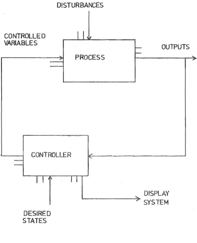
Put simply. a process can be considered as a black box (Fig. 1.1).

The process has two classes of inputs; non-controllable, which are

called disturbances, and controllable, some or all of which are used by

the control system to counteract the deleterious effects of the

di sturbances. Some of the outputs from the process wi 11 be exami ned by

the control system to determine the state of the process. These are

compared with, or the computed resultant state is compared with, the

optimum 'set by other controller inputs. Any difference causes the

control system to alter the controllable process inputs so as to move the

process closer to the optimum.

The control system has another function concomitant with maintaining

the process at its optimum and that is information presentation. The

process engineer and the process operator must be kept informed about the

current state of the process. This may be achieved by displays on

DI5T URBANCES

CONTROLLED

I

11V

VARlABLES

_ .... _PROCESS

.--::..

-CONTROLLER J

I '

=

I I

I ~

DESIRED STATES

I I

to-- OUTPUTS

F-" DISPLAY , SYSTEM

FIG 1.1 SIMPLIFlED

CONTROL

SYS TEM

[image:9.595.114.508.145.631.2]

chart recorders and panels on the front of controllers or, with modern

technology, through VDU's (visual display units) and line printers

connected to a computer.

1.2 Justification for Process Control

The equipment required to effect process control, the sensors,

controllers, final control elements and such peripheral services as these

use cost from 6% to 30% of the processing plant (1-5). As with any other

expenditure this must be justified. Qualitative justification has been (1-5)

- a reduction in labour

- increased production

- improved and more uniform product quality

- reduced consumption of raw and process materials

- less plant maintenance under less severe operating conditions

- reduced utilities and energy consumption

capital savings through

- elimination of intermediate storage

- reduced inventory

- less excess capacity

- increased yields, minimum waste

faster readjustment of the process to variations in raw materials

or operating schedules

- increased plant and personnel safety

It is possible to directly quantify some of these factors, for

example, reduced labour and plant requirements, savings on raw materials,

utilities and energy and increased yields. It is also possible to place

a value on those factors not so directly quantifiable, A plant

be Pl and with control this could be reduced to P2. The saving is there-fore $x(P1 - P2). This statistical argument can also be applied to increased product uniformity (1-5). These savings are then offset

against the cost of the control system to decide if its use is economically

justified.

1.3 Development of Process Control

Initially, process control consisted of sensors and their accompanying

indicators or recorders geographically distributed around the plant. Large

numbers of operators were required to monitor these and make the necessary

adjustments to the control elements. Automatic controllers were developed

because of the large variability in results between operators and in fact

for the same operator depending on work load, time of day, mood etc.

These controllers, P, PI or PIO were still spread around the plant and

during fault conditions an operator could still oversee only a small

number of them.

To improve the efficiency of the operator, the next step was the

I

design of centralised control rooms. The readings from sensors

distributed around the process were fed to controllers housed in these

control rooms and the resulting control action returned to the actuating

element. The control rooms, typically, had the controllers spread along

one wall, and while the operators now had their information close at

hand, the volume presented resulted in important changes being missed.

The use of human factors engineering, or ergonomics, to optimise the

presentation of this information improved the situation. By logically

grouping the information, using consistent displays and removing

non-useful detail the workload on the operator was reduced. However, under

high stress conditions information could not be assimilated quickly

Human factors engineering, or the design of work situations to

human capability constraints, was able to make further improvement

when digital computers became cheap enough to allow their use in control

rooms. This permitted the adoption of the "management by exception"

pr"inciple to reduce operator overload. Parallel information presentation

overwhelmed the operator by constantly displaying all available information

about the process. Management by exception meant that the operator was

only presented with information he needed at that particular time. This.

combined with an alarm panel. significantly reduced the operator's load

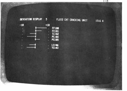
without reducing his efficiency. Figure 1.2 shows a typical operator

display panel from Foxboro's IMPAC system (1-6). Figure 1.3 shows the

same for a later model Honeywell VUPAC (1-7).

Because of their still high cost, the computer could not be justified

solely in terms of man-process interface improvements. The machine was

also time-shared around the control loops for either supervisory or direct

digital control and data logging. This situation was far from satisfactory

however. because computer failure meant loss of all loops. To reduce the

catastrophic effect of this, the most critical loops had conventional

analog controller backup. System reliability could be "improved by using

several computers, either reducing the area of responsibility of each or

using the extra intelligence in a back-up mode. Here again, cost becomes

a dominating factor and typically these types of computer control systems

were and still are used only in highly critical areas, e.g. nuclear

reactor control.

A solution through cheaper computer power became available with

the advent of the microprocessor. Now it was poss"ible to have many small

computers, each responsible for as few as eight. or in rarer cases one.

control loops. By distributing the microcomputers around the plant,

L'J

-Ul

Q

•

0-..IJ

o

-~

!

::

c:.

L!J

-0

•

Ul

i:! ~

w

rn

0

G

1-7

w

u

0

LE

•

0:::

w

Ul

Ul

0::: I... W

~

a..

" N .:.

D

~i ~

_..

"

_...

-m

[image:14.594.92.537.34.353.2]

transmission, such as noise were easily solved. Inter-computer

communi-cation was achieved over a twisted pair or coaxial cable, in one of three

basic configurations (Fig. 1.4) i} a star

ii} a multidrop line

iii) a ring

The commercially available systems use variations or combinations of all

three types.

1.4 Present Systems

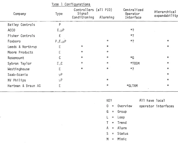
Table 1.1 shows a list of the offer"ings commercially available at

the time of writing. The table "includes information about the controllers,

the operator interfaces and, where appropriate, comrnunications rnethods.

These systems have been sorted into three categories based on their

operational configurations (1-8).

Type 1 systems are the conventional centralized control room layouts.

Sensor readings are brought into the control room and the output from the

controller fed back to the actuator.

The multidrop line and the hierarchical star configurations make

up Type 2 systems. The advantage here is that level sensor signals

have less distance to travel to the controller and thereby suffer less

from the effects of noise. There is also greater use of the operator

interface using the Imanagement by exception ' principle (see section 1.3).

The last configuration, the ring, is the least used. There is only

one control system, the System 1100 by Xomox, that uses it. Data

transmission is uni-directional around the ring and hence reliability

1 Configurations

Controllers (all PID) Centra 1 i zed

Hierarchical

System Company Type Signal Operator _{expandability}

Conditioning Alarminq Interface

7000 Bailey Controls P

Bristol UCS3000 ACCO E,lJ P *?

ac2~ dc2 sher Controls E *7

Spec 200 Foxboro P ,lJP * *? *

Centry Leeds & North rup E * * *

Synchro 350 Moore Products E * *

Diogenes Rosemount C * * *G *

III Sybron Taylor E,C * * *TOSM *

Veritrak Westinghouse E * * *? *

NAF-Unic Saab-Scania *

PCS 700 NV Philips llP * *

Protronic Hartman & Braun E * *GLTAM *

KEY All have local

p _{= Pneumatic 0} = Overvi ew operator interfaces

E = Electronic G = Group

= M, croprocessor L

=

Loop

C = Computer T

=

Trend

A = Alarm

S

₌

Status

[image:16.841.203.788.64.532.2]

(baud)

OGL

_*

Current loop ? ? Star

AGL ? Multidrop

ROGLA

_*

Coaxial 1.5M 5000 ft Multi drop

TGO

_*

Current loop Star

?

_*

? ?

OGL Coaxial or 600 ft ?

twisted pair

AOLMR Twisted pair 500k ?

TG

_*

? ?

AGLT

_*

Coaxial 10 km Multidrop

OGLTM

_*

30 core cable Star

?R ? 250k ?

OGLA

_*

? 1000 ft Multi drop & Star

?GR

_*

? 15k ft Multidrop

OGR

_*

Coaxial 1M Multidrop

OGLTR

_*

RS232 300-l9,2k Star

MTLA 10 rnA 1200-9600 3-.6 mil es Star

?G

_*

Coaxial 1 ~1 3-4,5 km Multidrop

1M 1 .5 M 4 km Multidrop

OGLAM

_*

Twisted pair 500 k 1500 m l'1u1 ti drop

? Coaxial 500 k ?

Twisted pair 250 k 2 km Multidrop

See Centum RS232 10 km Multi drop

TTY Ring

Key (Di s plays)

0

=

Overview

G = Group

L = Loop

T = Trend

A

=

Alarm

S = Status

STAR

MULTIDROP LINE

RING

1.5 Objectives of this Research

In view of the decreasing cost of computing power, the idea of

distributing intelligence around the plant and providing a communications

highway would become more prevalent in available control systems. This

research aimed at outlining the requirements of these systems with

special attention given to the problem of the man/machine "interface.

In the following chapters the computer based distributed control

system ;s first analysed to show the subsystems that are a part thereof,

and then each subsystem ;s examined in greater detail. The final two

chapters discuss a system that the author constructed based on the above

information and the areas that could be improved with the availability

REFERENCES

1-1 Handbook of Industrial Control Computers

T.J. Harrison, Wily-Interscience, 1972.

1-2 Man and Computer in Process Control

E. Edwards, F.P. Lees, I.Chem.E., 1972.

1-3 IIComputerized Process Control in the Steel Industry"

Review 224, International Metals Reviews, 1977, pp.355.

1-4 "Control Equipment Developments Lead to a Future of Distributed Controll!

E.J. KompQss, Control Engineering, December 1977, pp.35.

1-5 "The Justification of Expenditure for Process Control Equipment"

R.M. Allen, ACIS 8th National Conference, Auckland N.Z., 1977.

1 Fox 2 Process Computer Systems, Impac Software, System Product

Specification SP-53000AX-A

The Foxboro Company, December 31. 1971, pp.IS35, IS37.

1-7 Vupak Systems Manual

Honeywell Inc., 1974.

1-8 liThe Configurations of Process Control: 1979"

Control Engineering, March 1979, pp.43.

1-9 "Internati ona 1 Manufacturers Offer Many Choi ces in Process Control

Systems"

Kenneth Pluher, Control Engineering, January 1980, pp.54.

1-10 "Distributed System is ExpGndable from Eight Loop"

Henry H. Morris, Control Engineering, June 1980, pp.78.

1-11 II Introducing Four More New Integrated Di stri buted Control Systems II

Kenneth P1uher, Control Engineering, August 1980, pp.41-.

1-12 "Foreign Distributed Control Systems Keep Pace with Industry's Needsll

2.1

2.2

CHAPTER 2

SYSTEM ANALYSIS

Functional analysis

Economic analysis

2.2. 1 Hardware cost

2.2.2 Software cost

2.2.3 Wiring cost

2.2.4 Failure cost

2.2.5 Concll,lsions

Fi gures

2. 1 Multidrop hardware layout

2.2 Hardware cost

2.3 Software cost

2.4 Wi ring cost

2.1 Functional Analysis

A functional analysis of any system involves answering the question,

"What does the system do?" A distributed computer based process control

system is designed to maintain a process at its optimum operating condition.

"Maintain" implies the system must have a high reliability and 1I0pt"imumli

includes consideration of economic, safety and legal factors. Having

broadly stated what the system does, the next question to be answered is,

IIHow does it do this?".

To fully answer the second question, and thereby the first, we must

break down the complex control system into its sub-units. These sub-units

are then divided further until we are reduced to parts small enough to be

explained in complete detail.

The type of distr"ibuted control system being studied has three

separate interfaces with the world

i) the process interface

ii) the engineer's interface

iii) the operator's interface

In systems with extensive report generating features. a fourth, the

management interface, can also be defined.

The control strategy is implemented through the process interface.

Sensors feed data to the control stations enabling the current state of

the process to be determined. This state is then compared with a model

stored in the microcomputer and any difference is used to calculate the

action required to return to optimum. This action is then sent to the

final control elements; valves, motors or heaters. In addition, checks

on the approach of variables to safety and other constraints can be made

The engineer, in designing the control strategy, enters information

into the computer through his interface, enabling the computer to

determ"ine the state of the process and to calculate any action required.

A constant check on the state of both the process and the control

system, and entry of data to fine tune both parts, is achieved through

the operator's interface. Because of its critical function, the control

system's success or failure as a whole depends on the careful considered

design of this interface.

These three interfaces, or windows to the world, make up the

presentation sub-unit. The second sub-unit that can be identified is

the database or storage unit. The engineer's information, the control

parameters, and the data collected from the process are stored in a

data-base. The input from the operator's interface involves making adjustments

to variables in this database. Its design affects the engineer's

inter-face and thus the useability of the whole system and also its effectiveness

as a control unit. The more efficient the database, the faster the system

can respond to process changes. As a result, the database is viewed from

two levels, the process interfaces with the physical storage of information

and the engineer with logical storage of the same information.

In operation, data transfers of three types will be occurring

-i) storage-storage

ii) storage-presentation

iii) presentation-storage

These are made through the communication subsystem. Use of the communication

channel for storage-storage transfers is necessary because of the

distributed nature of the system. To fulful the reliability criterion, the

control intelligence is not concentrated in one machine but distributed

among several microcomputers. Consequently the database will also be

The communication subsystem is designed so as to minimize the cost

of the overall scheme. Depending on the price of computing power, the

resulting configuration will be a star, a ring or a multidrop line (see

Fig. 1.4). If an economic analysis shows a small number of loops per

processor to be optimal, the ring or multidrop line is preferred, while

a large loop to processor ratio favours the star format. This is because

of traffic density on the data highway. In the communications subsystem,

consideration must be given to the physical unit, i.e. a twisted pair, a

coaxial cable or an optic fibre, and the logical unit, i.e. the message

format, error correction-detection scheme and the handshaking convention.

So we can now say that a distributed computer based process system

is made up of the following subunits

1) the communication system

ii} the distributed database

iii} the presentation system to the a) process b) engineer

c) operator

It is also possible to consider the hardware subunits. These are

the control station, the engineer's interface, the operator's interface,

and the database and communication controller. Figure 2.1 gives a

typical layout for the multidrop configuration.

2.2 Economic Analysis

Having completed a functional analysis, an economic analysis is

necessary to answer the question, "How distributed should the system be?",

and then decide which of the three poss"ible configurations is more appropriate.

To do this we need to find the most economic number of control loops for

each microcomputer, or minimize a cost function with respect to the number

ENGINEERS

INTERFAct;

OPERATORS

INTERFACE

CONTROL STATIONS

The cost of a system includes

i) _design

ii) computer hardware and software

iii) wiring

i v) install ati on

v) failure

This analysis only considers the analog control system as for any

particular situation the digital control system, best implemented through

modern PLe·s (programmable logic controllers), can be considered as a

fixed cost. The logic control system will be required regardless of the

number of loops that will be implemented in each microcomputer. If we

assume a system with

N microcomputer based control stations

n inputs

and m outputs

where m is fixed at n/2, the same as that used for the Honeywell TDC2000

design, then for a fixed value of n, and therefore m, we vary N to

minimise the cost. It is only necessary, therefore, to consider those

factors that vary with N as a 11 others wi 11 effect; ve ly be only a fi xed

additional cost. From our original list, then, we may ignore design and

installation costs which leaves four sections

-; ) hardware

ii) software

i; i) wiring

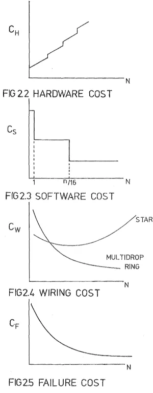
2.2.1 Hardware costs

Hardware cost

=

CPU + memory + input/output +

power supply + box, cabling, etc.

Let H

=

CPU + power supply + box, etc.

Now memory comprises program and data memory, i.e. ROM + RAM.

The program memory will be of fixed size, but the data memory will have a

fixed requirement plus extra for control loop data storage. If we allow

5k bytes of memory for the storage of program and set data, and allow .5k

bytes for each control loop, the ,memory requirement becomes

(5 + .5n/N)k bytes

The input/output subsystem includes the communication system, process input

and process output. If we now let

HI = H + communication system

then the hardware cost per microcomputer

=

H" + (10 + _R)*Cm +

[~J*CDA

+

~

* Co

where H" the cost of HI

C_m = the cost of .5k bytes of memory

C

OA = the cost of an eight channel data acquisition module

CD = the cost of a D/A converter

R

=

the number of inputs per microcomputer

=

n/N

and [J = the ceiling function.

Therefore, the system hardware cost

C

H = (H" + 10*C )*N m +

[~J

* C * N OA + R * Cm * N +

R

2 * C * 0

=

(W + lO*C )""'N _m + [-'!] "'" _{8 CDA} + n * C_m +

2-

_{* Co}

I~

2.2.2 Software costs

In every microcomputer there will be a set of standard

routines that are used to effect the control" These will be the same

for each control station and so will not affect the cost function. The

software costs that should be considered are those of a load sharing

routine, to even out the number of inputs scanned each interval, if the

number of inputs per microcomputer becomes too large, and if only one

large machine is used, a comprehensive multitasking executive. If we

assume the basic routines cost S, the load sharing routine for greater

than 16 inputs per microcomputer is SL' and the multitasking executive

for N = 1 is SE' the result is shown in Figure 2.3.

2.2:3 Wiring costs

Let us assume that the microcomputer based control stations

lie on a circle of radius D. The inputs to each station will be connected

in a star configuration and can be approximated to lie on a circle of

radius r about that station. Then the length of cable needed to join

the control stations is ND for the star

1

2nD(1 -

w)

for the multidrop line

and 2nD for the ring,

and the length of wire needed to join the inputs to their respective

station is nJ. As the number of stations gets larger each input will be

1

closer so raN' say

nr * N

N

r

=

*.

Therefore the wire for all input is

kn

= ₁₁

If the wire for joining the control stations costs x per unit length

and for the inputs y per unit length, the total wiring cost is

C_w = _{ND +} ~ star

x N

2nD( 1 1 ~ multi drop 1 i ne

= _{- W)x} +

N

= _{2nDx +} kny ring

c.f. _Y - . aN + _N b star

::: a + b multidrop line or ring

N

(see Fi g. 2.4).

2.2.4 Failure costs

Let the cost of failure of a single control loop be c per

hour. If the number of loops for control station is

N'

then the cost

of microcomputer failure is ~c per hour. Assuming a negative exponential

failure distribution (2-1) and defining

F ::: mean time to failure

R ::: mean time to repair

T ::: operating life in hours (» F),

the downtime of a microcomputer is

RT

R + F hrs.

Therefore the cost of failure is

nc

*

RT

N

R + F

Now ncT is the cost of failure of all loops for the operating life of

the control system. This is equivalent to having no control at all, and

under these circumstances the plant will cease to be profitable. Therefore

ncT equals the profit of the plant, say P. The cost of failure then

becomes

.!:

;Ie R

N R + F

and for all control stations

::: P

*

R R + F

which is independent of N.

However, as the number of control stations decreases, the

number of components used to construct each station will increase and

a and b are constant and x is the number of additional components required.

Then the cost of failure

R CF

=

P

*

R + (a - bx)

c.f. y

(see Fi g. 2.5).

2.2.5 Conclusions

To determine the optimum number of inputs per control station

(or the optimum number of stations for the system), the total system cost

must be minimised. As stated in section 2.2, this total cost, considering

only the parts that vary with the number of control stations N, is

Total cost

=

hardware + software + wiring + failure.

The equations were programmed on a computer using the following

data:-Hardware costs based on current N.Z. retail prices

Hit _$1,000

C :::: $50

m C

OA = $150

Co ::: $10

ii) Software costs

The loading sharing routine is approximately 500

statements long (as designed by the author) and the executive

(based on the POPll RT-ll system) ;s 2000 statements. At a

cost of $6 per statement (2-2), the costs are

SE

=

$12,000

\ ::: $3,000

iii) Wiring costs

FIG 2. HARDWARE

COS T

FrG

I I

1

I

I

I

I I

OF WAR

T

N

N

STAR

MULTIDROP

- - " RING

N

FIG2.4 WIRING CO

T

N

[image:31.597.122.423.50.819.2]

of diameter of the order of one kilometre, as D ::: 1000.

Coaxial cable, for inter-station connection is $1 per

metre on current costs and for input connection, cheaper

wire of 30¢ per metre is adequate. For the sake of

simplicity the constant k is set equal to D.

iv) Failure costs

The profit of a plant can be considered as the return

on an investment equal to the capital cost of that plant, so

where n = plant life in years, 15

r

=

effective rate of return, 15%

A

=

capital cost, $lOS

Therefore P ::: $S.14 x lOS.

The mean time to repair a modern computer board is of the order

of one hour so R ::: 1. The mean time to fa"j 1 ure of the same

;s 1000 hours, and considering the extra complexity each

additional chip will reduce this by 5 hours. Strictly speak"ing

this time is not constant and will exponentially decrease but

for the range considered in the program it was assumed linear.

The results are shown in Table 2.1.

The first important conclusion ;s that the star

configura-tion is never the most economic. The difference between the

multidrop line and ring format is not significant and these

have been included in the one column. The ring suffers from

reliability (see Chapter 6) without the addition of intelligent

Inputs Optimum Inputs/pC Total Cost Star Mul drop ne Star

40 4 3 9.19 x 10 5

80 5 4 9.44 x 105

120 6 5 9.65 x 105

160 7 6 9.83 x 105

200 8 7 9.98 x 105

240 8 8 1.01 x 106

280 8 8 1.03 x 106

320 8 8 1.04 x 106

360 8 8 1.06 x 106

400 8 8 1.08 x 106

Multidrop Llne

9. 14 x 105 9.34 x 105 9.50 x 105 9.65 x 105 9.78 x 105 9.90 x 105 1.00 x 105 1.02 x 105 1.02 x 105 1.04 x 105

N

I

...

The range of inputs considered was a minimum of 40 to a

maximum of 400 per system. The optimum always lay between

2 and 16 inputs per microcomputer and so neither extra

soft-ware routines affected the cost. The most significant cost

was the failure cost, contributing as much as 90% of the total

cost in some cases. The wiring and hardware costs were of a

similar order and for the largest system were only 40% of the

overall total. Ignoring the failure cost completely moved the

optimum to more inputs per station. stopping at 16 because

REFERENCES

2-1 System Reliability Engineering

G.H. Sadler, Prentice Hall, 1963.

2-2 'Focus on Software'

3.1 Function

3.2 Hardware

3.3 Software

Fi gures

3.1 Process interface

CHAPTER 3

PROCESS INTERFACE

3.1 Function

The process interface has two identifiable functions. The first is

to effect the control strategy as defined by the engineer. The second is

to collect and process data for use by the process operator in his role as

supervisor, or by the engineer, in reports or higher level control

calculations. The interface must therefore be able to capture this data,

convert it to a form suitable for use by the microcomputer, process the

result using the available software routines or computer language, and

finally output the desired control action and convert it to a signal

capable of driving the control actuating device (Fig. 3.1). The hardware

components, including the microcomputer, are discussed in section 3.2 and

the software requirements in section 3.3.

3.2 Hardware

What must the hardware section of the process interface accomplish?

It must measure the physical variables of interest, convert these to an

electrical and/or digital analogy which can be used by a microcomputer

based controller. On the output side it must do the reverse. The nun~rical

value from the ~C is changed to a signal suitable for actuating the final

control element.

The input can be considered as having four separate stages (Fig. 3.l):

i} the transducer

ii) pre-multiplexor conditioning

iii} the multiplexor

iv} sample and hold/analog digital converter

Table 3.1 lists the more common process variables and means of measurement.

It should be noted that not all are real time methods and some do not give

TRAN SDUCER AMPLIFIER I MUX

FILTER SAMPLEI

HOLD

AI

ACTUATING ELEMENT

3.1

P 0 ESS I T R

I I

I FILTER

I I

I

I OUTPUT

I

PROCESS

I

I

L!NEARISING

.. .- &

SCALING

ALARMING

CONTROLLER

W

The particular choice of transducer depends on three factors;

i) economy

ii) safety

iii) accuracy, relative and absolute

Economic constraints are important but are not the overriding criterion.

Safety aspects may preclude the use of certain transducers. For example,

it may be necessary to convert a level measurement to a pneumatic signal

first because the presence of an electrical signal may constitute an

explosion hazard. Transducer accuracy is affected by its two basic parts.

To measure a variable, the transducer compares the incoming signal with

some previously determined standard. The quality of this reference affects

the absolute accuracy of the measurement and the comparison affects the

relative accuracy. So it is possible for the device to be consistent

(precise or relatively accurate) but to give a poor indication of the state

of the physical variable (inaccurate or poor absolute accuracy). The

resolution of the comparing mechanism will also affect accuracy. Low

resolution means the available scale is divided into very few stages giving

a coarse measurement.

Having eventually converted the process variable into its electrical

analog, the signal must be prepared for computer use. If the computer ;s

any distance from the measurement point, the signal must be transferred.

This transfer gives rise to a large number of errors. To reduce the effect

of noise on the signal it should be amplified as soon as possible. This

amplification must take into account such problems as common mode error

sources, normal mode error sources and the major causes of these. Common

mode errors are, typically, voltages that are in parallel with the desired

signal. These can arise due to ground loops or induction between the Signal

carrying wires and nearby power sources or users. Normal mode voltages are

Table 3 Process Variables and Measurement Systems Temperature

Thermocouples

Resistance thermometers Filled system thermometers Liquid-in-glass thermometers Bi-metallic strips

Optical pyrometers Pressure

Flow

Liquid column

Elastic element methods Bou rdon tube

Bellows Diaphragms Electrical methods

Strain gauges Piezoresistance Piezoelectricity

Variable head meters Variable area meters

Positive displacement meters Turb i ne meters

Mass flowmeters Sound reflection Light reflection Wei rs

Flumes

Level

Visual gauges Float actuated Oi sp 1 acer Head

Electrical methods Resistance Capacitance Sound reflection Nuclear radiation Light reflection Thermal conductivity Physical Properties

Density and Specific Gravity Li qui d col umn

Displacement

Di rect mass

Radiation absorption Viscous drag

Viscosity

Viscous drag Refractive index

Transmission Reflectance

Thermal conductivity Boiling point

Table 3.1 contd.

Chemical Composition

Chromatographic analyzers

Infrared analyzers

UV and visible analyzers

Turbidimetry

Paramagnetism

Moisture

Dew point

Electrolysis

Capacitance

Heat of sorption

Piezoelectricity

Psychrometry

Conductance

Karl Fischer method

Electroanalyticity

Conductance

Capacitance

Potential

pH

Specific ion probes

may arise due to resistive drops in signal wires, thermocouple effects

when dissimilar wires are joined and, again, ground loops. Common mode

problems can be solved, or eased, by using instrumentation or isolation

amplifiers, (3-3), or early digitizing, but correction of normal mode

errors can only be effectively done by careful design to remove their

sources. The amplified signal will still have some noise and this can

be reduced by filtering. In addition, the use of a filter can prevent

aliasing or errors due to freque~cy folding. Aliasing is caused by high

frequency components of the signal. A slow sampling rate can cause the

computer to react to harmonies of these higher frequencies, instead of

the signal of interest. Frequency folding is an effect caused by the

reflection of the higher frequencies about a point equal to half the

sampling frequency. If the highest frequency in the signal is fh and

the sampling rate if f

s' then if (fs - fh) is less than fs/2. there will

be a resultant frequency folding (3-11), Typically, a low pass filter

with a cutoff frequency as low as possible, commensurate with the

band-width of the signal of interest. is used, but specialized filters such as

notch filters, synchronous filters or derivative controlled filters may

be required in some situations. For example, where specific noise spikes

occur (notch or synchronous filters). or where there may be a speed of

response requirement (derivative controlled filters) (3-3).

Primarily for economic reasons, the now amplified and filtered signal

is fed to a multiplexor (MUX). The use of a MUX means that only one analog

to digital converter (A/D) is needed for many incoming measurements. The

MUX is a set of switches that can be selectively turned on to connect only

one measurement line to the A/D. The switches can be mechanical, as in

relays, or semiconductor, as in FET switches. The problems in using a

i) leakage, due to off resistance being less than infinite;

ii) crosstalk, the off channel affects the selected channel

giving common mode problems;

iii) switching time, affecting the possible sampling rate.

The last step before the computer is

AID

conversion. The choice

of converter is critical to the whole measurement. Its resolution,

accuracy and speed affect the final result.

There are two basic types used in process control, an integrating

AID

and a successive approximation type. The integrating converter

integrates the incoming signal for a set time linterval and then measures

the time required to ramp the result back to zero at a fixed rate.

Typically they are only used in low speed applications. The successive

approximation variety compares the signal to an internal voltage created

by successively turning on bits in the resulting word and leaving them on

or switching them off after comparing the two values. They are much

faster and have the capacity for high resolution. However the

AID

is

typically not fast enough to convert the signal without it having changed

appreciably during the conversion. For example. a 12 bit

AID

that had

a conversion time of 24 ~secs could only handle a signal of 1.6 Hz. To

overcome this problem a sample and hold unit is used before the

AID

to

sample the signal and hold the result for the

AID

to convert. If it is

necessa~ to sample a large number of channels simultaneously, the sample

and hold unit may be placed before the MUX. Accuracy in an

AID

is

dependent on its linearity, as zero and full scale offset voltages can

be trimmed with a resistance. A typical specification will quote a total

non-linearity of plus or minus a fraction of the least significant bit

and at any stage the output should be in error by no more than this. The

process variable has now been measured and converted to a computer useable

voltage to frequency converter may be preferable with the result being

measured by a pulse counter. This can reduce, in some situations, the

effects of some of the errors we have discussed.

After the software has processed the input, its digital result must

be delivered back to the \~Jactuating device. The necessary conversion is

done by the output hardware. The first step is to convert the digital

result into form acceptable to the actuator of the final control element.

This may mean conversion to an electrical value via a digital to analog

(D/A) converter, or to a form of modulated pulse output.

The two main types of digital to analog converters are the weighted

current source and the R-2R ladder network. The weighted current source

D/A has a series of transistors whose collector currents are set by

resistors with values of R, 2R. 4·R etc. The transistors are switched on

or off according to the appropriate bit in the output word. This method

is fast and simple but the large range of resistance values required for

high resolution results in significant temperature effects. The R-2R

network has a series of resistances that are either in series with the

output of values R or shunt across the output with values 2R. The shunts

are connected to earth or a voltage source depending on the bit value of

the output and the division of current as it flows down the ladder results

in the required output. This method requires twice as many resistors as

the weighted current source but all are of value R or 2R and so are better

matched. Other advantages are that the output amplifier always sees a

constant input resistance and the resistance values can be kept low to

ensure low power consumption and high speed.

The pulse output systems can be modulated in one of four ways:

i) ampl i tude

i i ) frequency

iii ) durati on

For computer output that represent the absolute value of the control

element, amplitude modulation tends to be the most common as it is the

least complicated to implement. For change in position output»any of

the four methods can be used.

This conditioned output is then transmitted to the actuating element

of the controller hardware. Table 3.2 lists common actuating methods and

final control elements {3-2}. As with the input)the use of pneumatics or

hydraulics is typically for safety reasons although with some output _.1

situations) they may also effect a large amount of power amplification.

The remaining hardware unit in the process interface is the control

station, or microcomputer, itself. Its primary design consideration is

reliability. Less important criteria are performance, cost and modularity.

The three functions it must perform are control, communication and the

provision of a local man-machine interface. To some extent these are

independent and it is therefore possible to allocate each to a separate CPU,

fulfilling all but the cost restriction. However it is cheaper to use

only a dual CPU system with little or no loss in performance, modularity

and reliability. Figure 3.2 shows the result.

Reliability, and reconfiguration should a fault be detected, are both

accounted for. The control interface CPU is capable of stand-alone

operation and the unit as such could be used as a multi loop controller.

Therefore communication system failure should not affect control

Should the control CPU develop a fault, the communication CPU, through the

duplicated process inputs, can send the measurements to a standby CPU with

the results being sent back for output. This reconfiguration should take

place in less than ten sample intervals and if the communication channel

is fast enough "in less than a second. The layout is therefore dynamically

reconfigurable giving a very high reliability for small cost (redundancy

COMMUNICATION HIGHWAY

PROTOCOL CHIP

DMA

LOCAL

RAMIROM

COMM CPU

COMMUNICATION BUS

-

_COMMON

RAM

PROCESS INTERFAC

I

-PROCESS

CONTROL BUS

CONTROL

1 - - - 1 CPU

LOCAL

1 - - - 1 RAM/ROM

LOCAL ,;

_l-...j INTFACE

standby controllers).

The other criteria are also satisfied with this design. Cost is small, as explained above, the only extra requirement being fast access memory so the CPUls can interleave their read/write cycles. Performance is enhanced by using dedicated intelligence for each function and the modularity constraint is complied with as explained above.

3.3 Software

The software requirement for the control station can be divided into three categories:

i) real-time executive

ii) control based applications software iii) communications software

The communications software will be discussed in Chapter 6 and the local interface section of the applications programs will be covered in Chapter 5.

The basic functions for a real time executive for the ~C control station are:

i) task initialisation and scheduling or rescheduling ii) intertask communication and synchronization

iii) timing

iv) interrupt handling v) input/output handling

In this context I/O handling tends to be very situation specific and covers both process I/O and human I/O. Process I/O includes control of the

receipt of an interrupt, polls each possible device in turn to determine

the interrupt source. The timing function must be external to the CPU

to ensure some absolute measure of real time. Task initialization is

usually based on the timer input as the tasks in question are typically

the control routines. Task scheduling or rescheduling may be necessary

to alleviate uneven CPU loading. The final function is intertask

communication. This may occur within a CPU or if external to (or across)

CPU's may make use of the communication system. Because in the process

control situation the number of tasks is limited (see Chapter 2),8 inputs

per CPU, the executive in a control station is uncomplicated and

conse-quently reliable~ fast and compact.

The applications software is composed of a series of routines which

are used to effect the software processing between input and output

(Fig. 3.1), The engineer will specify the routines to be used for each

input and the list produced, be it a program written in some process

control language or literally a list of routine calls, constitutes one

task under the executive. A basic collection of programs would cover:

;) a software filter

ii) linearizing and scaling routines

iii) alarm checking

iv) control routines

v) output checking and formatting.

The hardware filter will have removed most higher frequency noise

from the signal, but the data may still need to be smoothed. The most

common technique is the exponential filter, a simple first order lag.

where Y

t _n = present output

Y

t = previous output

n-l

x

= input

a· = filter constant = Ts

TF

TS = sampling interval

TF

=

fi lter time constant

With a set to one, the output equals the input. As a gets less, so less

of the new input and more of the previous output is used, the system

becomes more sluggish, until at a value of zero the input is not used

at all, The recommended range for a is 0.7 to O,g, There are other

possible filters that introduce less phase lag but the computational

requi rement becomes too great (3-9),

Linearizing routines cover just about every mathematical possibility.

For example, a pH signal may need an inverse sinh function, a flow meter

based on pressure drop uses a square root function, and thermocouples

may require a high degree polynomial (or large look up tables). Once

linearized, the signal is then converted to engineering units by a

simple scaling:

Y ::: AX + B

where Y output

X ::: input

A = scale factor

B = offset

Alarm checking covers absolute alarms, with and without a deadband,

offset alarms (relative to some setpoint) or deviation alarms to check

rate of change. The deadband is used to ensure noise does not cause

multiple alarms when the process variable is hovering on an absolute limit.

Control routines include PID algorithms that output absolute values

that have variable gain or may have remote setpoint facility for cascade

operation. Refinements include bumpless transfer when changing from

manual to automatic operation and back)set point tracking for cascade

controllers, and the ability to incorporate interlocks and overrides in

the control scheme. Other control routines w'j 11 be needed for deadtime

compensation, feedforward control and derived variable control.

The output checking facility is used to limit the range of the

control variable. It is also used to keep the rate of change to a level

acceptable for the control element actuator. A side benefit of the rate

of change limit is that a CPU malfunction cannot affect the process too

quickly, hopefully not before the error has been corrected.

The range and complexity of the software processing options can

cause confusion for the process engineer. His method, of implementation

of these routines has a direct bearing on how they are written for the

Table 3.2. Final Control Elements

Linear Position Actuators

Pneumatic

Electropneumatic

Hydraulic

Electrohydraulic

Electric

Mechanical

Variable Speed Drives

Variable Electric Power Actuators

REFERENCES

3-1 Chemical Engineers Handbook, 5th Edition, pp22-33.

R.H. Perry, C.H. Chilton, McGraw-Hill, Kogakusha, 1973.

3-2 Ibid. pp.22-87.

3-3 Transducer Interfacing Handbook

D.H. Shingold, Analog Devices, 1980.

3-4 Analog/Digital Conversion

D.H. Shingold, Analog Devices, 1972.

3-5 "Consider Every Error Source for Data Acquisition Design"

D. Chase, Control Engineering, June 1980, pp65.

3-6 "System Archi tecture Affects Data Acqui s i ti on Accuracy and Flexi bil ity"

D. Chase, Control Engineering, July 1980, pp83.

'3-7 IIData Acquisition Can Falter Unless Components are Well Understood"

D. Santucci, Electronics, November 13, 1975, pp.114.

3-8 "Manouvering for Top Speed and High Accuracy in Data Acquisition"

D. Santucci, Electronics, November 27,1975, pp.115.

3-9 Smoothing, Forecasting and Prediction of Discreet Line Series.

R.G. Brown, Prentice Hall, 1963, Section III.

3-10 "Designing and Programming Control Algorithms for DOC Systems"

E.H. Bristol, Control Engineering, January 1977, pp.24.

3-11 Electronic Design's Gold Book, Vol. 3

4.1 Function

4.2 Software

4.3 Hardware

Fi gures

CHAPTER 4 ENGINEER'S INTERFACE

4.1 Function

The engineer's interface is his means of communicating with the

control system. It differs, in this respect, from the operator's interface

which provides a view of the process rather than the control system. The

engineer has two primary tasks that he must accomplish through his interface:

i) configuring the control strategy

ii) initializing the parameters in the system.

Modification of the configuration or the control parameters is a secondary

requirement but still important.

For the engineer to make optimal use of the control system, the major

design consideration should be flexibility. It must be capable of

imple-ment-ing any and all of the engineer's control schemes. The most flexible

system available at present is to allow him to program his strategy in a

real time computer language. These range from extensions of Fortran and

Basic, to specifically designed languages such as RTL and Coral 66 (4-4).

The advantage of this flexibility is the use that can be made of process

knowledge. Full utilization can be made of feedforward control, derived

variable control and signal linearization to improve the quality of control.

However, the requirement that the engineer be a capable programmer is the

biggest disadvantage with this approach, although modern graduates'

experience with computing is fast removing this constraint. An improvement

in the situation can be made by providing, as part of the language, a

range of standard routines that the engineer would normally require in a

control scheme. This would include alarm checking. filtering, PID

controller algorithms, and others as mentioned in Chapter 3.

The other end of the spectrum in interface designs is to provide a

complete set of standard routines that, in effect, mirror the analog

components the engineer would have used. These are then joined using

but the tradeoff has been at the cost of flexibility. It becomes difficult

to provide those blocks that direct programming can account for, without

increasing the number of available blocks to the detriment of simplicity.

A system that uses the block approach is ABACUS (4-3).

To choose between these two extremes, we must examine the engineer's

approach to control system design. Typically, a control strategy is first

committed to paper as an instrumentation diagram, a graphical layout. The

problem arises when an analysis is done of the requirement of each

component in this diagram. If a block approach was adopted. what choice of

standard blocks should be made available to ensure adequate flexibility,

without over-complicating the interface. Harris and Bell (4-1) suggest

that the 22 signal processing functions of the SAMA RC 22-11-66 standaid

would be suitable. Perhaps the best criteria concept for deciding is that

of information chunking (4-5). Briefly, the more information contained

in each symbol~ the fewer symbols are needed to express an idea. For

example, using the decimal number system where each symbol represents a

choice of one of ten. the number 197 requires three symbols. In the

binary number system it needs eight, 11000101, and in hexadecimal only

two, C5. So while the 22 SAMA functions may be adequate, to improve

flexibility, it may be necessary to provide several refinements of one

function. Leeds and Northrup do this in the MAXl system by offering six

variations of the basic PIO algorithm (4-2). For the engineer to be

totally familiar with the possibilities of such a system. and thereby

be able to design any control strategy he wishes, is becoming not much

simpler than direct programming.

Another problem is providing, within the block algebra structure,

the capability of modifying any parameter, based on another input or the

output of some other block. Again, this is easily accomplished with a

To reduce the mental jump from the graphical layout to the computer

implementation, therefore, a combination of the two approaches would seem

best. Give the engineer the facility to represent the control scheme as

a series of functional blocks, but give him the flexibility to implement

a function of his own choosing within each block. if a suitable one does

not already exist.

The initialisation process can be completed at the same time as the

configuration ;s done, or it may be left so as to take advantage of a

data file that may be stored within the computer.

4.2 Softwa re

The information input by the engineer represents a set of files, one

per process input, that each contain a set ofrecord~. one per block. The

total is, in fact, a data base in the classical commercial sense. The

engineer's interface, therefore, represents one part of a data base

management system (DBMS). The design of a DBMS will then provide a

guide-line for the software required in the interface. The DBMS is more fully

covered in Chapter 7 but the relevant concepts will be stated here.

Typically there are two parts to DBMS interface software:

i) a data definition language

and ;i) a data manipulation language.

The data definition language is used to construct the logical storage

structure of the data (as opposed to the phys i ca 1) " Thi s has a 1 ready been

set by the method chosen for configuration, one file per input that

contains a header record and one record per block. The data manipulation

language is specifically what the engineer's interface software represents.

The language must do three things; create, modify and delete files. In

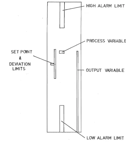
is best done graphically. Using a touch sensitive graphics screen, a

light pen or suitably interactive system, the engineer could select a

block, represented graphically by its standard symbol, and place it

within the structure as per the instrumentation diagram. Connections,

parameters, and functions if required, could be filled in as this was

done. The display could be as in Figure 4.1. Modifications and

deletions could be similarly handled. With only an alphanumeric VDU

the configuration and initialisation could be done in an on-line

conver-sational manner, using menu driven systems as per modern commercial DBMS

practise, with preformatted displays.

4.3 Hardware

From the previous discussion, the hardware requirement is:

i} a display unit

ii) an input system

iii} a back-up storage medium.

The display unit could be either a graphics terminal (high resolution

is not essential) or an alphanumeric VDU. With the graphics unit, some

sort of interactive input system is desirable, for example a touch sensitive

screen, and both display media require a standard keyboard for parameter

initialisation.

The back-up storage medium is needed to obviate constant data re-entry.

After a control station failure, the required information could be taken

off the back-up rather than re-entered by hand. Its possibilities range

from the expensive Winchester disc system. through bubble memory cassettes

GRAPHICAL LAYOUT AREA GRAPHICAL MENU

rD""

{jb

WORKSPACE &

PARAMETER INI TIALISATION

AREA

..

IG 4.1

NGtNEER

fNTERFA CE

REFERENCES

4-1 If Symbolic Function-Oriented Programming for Process Control Has

Simple Rulesll

L. Harris, 1. Bill, Control Eng-ineering February 1979, pp.91.

4-2 MAXl Controller Functional Description

Leeds

&

Northrup, 1980.

4-3 "Programming by Block Diagrams - a computer language to suit the

process engineerll

C.A.J. Payne, Canadian Control & Instrumentation, Dec. 1974, pp25.

4-4 Proceedings of the Conference on Software in Process Control

5.1 Introducti on

5.2 Function

5.3 Ergonomics

5.4 Functional Design

Figures

5.1 Subgroup symbol

5.2 Loop symbol

5.3 Loop trend graph