Method of increasing spatial resolution of the scanning near-field
microwave microscopy
R. Kantora) and I. V. Shvets
SFI Laboratories, Department of Physics, Trinity College, Dublin 2, Ireland
共Received 6 June 2002; accepted 25 September 2002兲
In this article we propose methods for the measurement of electric intensity of a microwave field above the surface of microwave circuits. Using miniaturized coaxial antennas and a special probe positioning system, we measure both the amplitude and the phase of the induced field above the device under test. We introduce a position/signal difference method to further increase the spatial resolution down to about 30m—about one order better than contemporary microwave scanning devices utilizing coaxial antennas. The effect is theoretically analyzed and experimentally verified. The probes are calibrated in a well-defined field standard to allow quantitative characterization of the measured field. Performance of our scanning system utilizing these methods is demonstrated using a PCB finger capacitor. © 2003 American Institute of Physics. 关DOI: 10.1063/1.1522486兴
I. INTRODUCTION
Contemporary systems for inspection of microwave cir-cuits are usually based on measurement of the signals at the device ports. In most cases they are limited to the measure-ment of the input and output signals. Such measuremeasure-ments are often not sufficient for characterizing the functionality of in-dividual elements and do not give a full description of dis-tribution of circuit signals. In some cases special measure-ment pads within the system are designed for direct coupling of the probes. Unfortunately, their use is limited due to rela-tively large contact areas, their influence on the circuit prop-erties caused by their high capacitance to the ground, cross coupling with other circuit elements and also the additional load of the measuring probes. These drawbacks effectively eliminate the use of such measurement techniques in highly miniaturized circuits, especially in microwave monolithic in-tegrated circuits 共MMIC兲. Due to the abovementioned rea-sons, noncontact scanning near-field measurements may be-come an attractive method for testing circuit performance and failure analysis. By analyzing the field distribution above the circuit surface one can evaluate not only values of the field sources 共charges/potentials, currents兲1,2 but also signal coupling between circuit parts, electromagnetic emission of the components of the device and other aspects of electro-magnetic compatibility.
II. ELECTRIC FIELD ANTENNAS
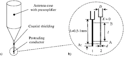
For acquisition of microwave intensities in a near-field region, short monopoles1,3or magnetic loops4,5 can be used for electric and magnetic field component detection, respec-tively. We have focused our attention on the measurement of electric intensity using miniaturized coaxial antennas— cylindrical short monopoles where a central conductor pro-trudes for a defined length from the shielding 共see Fig. 1兲. Our antennas are vertically positioned and, due to their axial
symmetry, they are sensitive to the normal component of the electric field intensity. The length of the protruding conduc-tor must not exceed the desired spatial resolution and in many cases it is chosen to be comparable or shorter than the diameter D of the shielding. Unfortunately, the antenna’s resolution does not just depend on the length of the protrud-ing conductor but also on the diameter of the shieldprotrud-ing sur-rounding it. Surface currents within the shielding also induce a secondary field and change the input signal. For well-defined antenna geometry the signal level can be evaluated using numerical simulation methods such as finite-difference time domain. As the result of the simulation depends on the particular field distribution, the external field is commonly assumed to be homogeneous, thus resulting in a single sen-sitivity coefficient, that is the ratio between the signal level and the field intensity.3When the field is highly concentrated around the apex of the protruding conductor, images with spatial contrast to a certain degree better than the length of the conductor and the dimensions of the shielding can be obtained. Unfortunately, those images lack good quantitative characterization as the antenna’s signal level depends on par-ticular distribution of the field that can no longer be consid-ered to be homogeneous. Additionally, the presence of the shielding close to the circuit may cause redistribution of the charges in the circuit and distortion of the primary field Ep.
III. POSITIONÕSIGNAL DIFFERENCE METHOD
It appears that only by decreasing the antenna dimen-sions along with coaxial shielding its spatial resolution capa-bility can be improved. Unfortunately, miniaturization of the antenna to the micrometer range makes its fabrication rather difficult, especially fabrication of the coaxial line of low di-ameter and the forming of a short protruding central conduc-tor. In this article we present a scanning method which over-comes the resolution limit determined by the antenna’s dimensions and allows us to increase its resolution capability without the need for further miniaturization of the antenna. Our antennas have a shield with an outer diameter of D⫽230
a兲Electronic mail: [email protected]
4979
m and a relatively long and thin central protruding conduc-tor: a copper wire of length L⯝0.5⫺1 mm, LⰇd, d ⫽8 m as shown in Fig. 1共b兲. The measurement method is based on comparing results of two subsequent scans with the antenna displaced by a small distance along its axis. We will show that for high density structures, when most of the field gradient is located close to the surface of the structure, the signal difference is determined only by the field strength sur-rounding the apex of the central conductor. By subtracting the two signals corresponding to two positions of the antenna displaced along its axis by distance ⌬z, one can cancel the contribution of the field in middle section of the protruding conductor, between planesAandBin the Fig. 1共b兲. Because for high-density structures the field above that region is sup-posed to be negligible, in this way the field surrounding the conductor apex can be isolated and measured. We shall call this method position/signal difference and we will show that it allows improvement of the spatial resolution of mapping of the microwave field.
IV. ANALYSIS OF THE METHOD
The antenna displacement is equivalent to changes in its geometry: reduction of the length of the protruding conduc-tor by⌬z and displacement of the front end of the shield by the same value. In order to show that the contribution of the external field from the middle section of the antenna can be suppressed, we will analyze the influence of the field and distribution of the currents induced in that region. Thanks to axial symmetry of the antenna, the analysis can be reduced to investigating the boundary condition at the center of the con-ductor. As the sum of the primary incident electric field and the secondary electric field induced by the antenna surface currents must vanish inside the conductor, the condition for longitudinal component of the electric field 共parallel to the antenna axis兲 before and after displacement of the antenna can be written as
Ezp共z兲⫹
冕
G1共z,z⬘
兲J1共z兲dz⬘
⫽0, 共1兲Ezp共z兲⫹
冕
G2共z,z⬘
兲J2共z兲dz⬘
⫽0. 共2兲Here the primary field at the conductor center Ep(z) and its z-component Ezp(z) do not depend on the probe position. The integrals in Eqs. 共1兲 and 共2兲 represent the secondary field
induced by the antenna as a sum of the contributions of the surface current elements to the z component of the electric intensity. The integrals are taken over the entire current space. J1(z) and J2(z) signify surface currents before and after the displacement, respectively. The Green functions G1,2(z,z
⬘
) represent the weighting coefficients of the contri-bution of current sources to the secondary field. For the pro-truding cylindrical conductor the coefficient does not change as a result of displacement along its axis as it depends only on the position of the observation point z relative to the position of the current source z⬘
G1共z,z
⬘
兲⫽G2共z,z⬘
兲⫽G共z⫺z⬘
兲. 共3兲Its explicit form is6
G共z⫺z
⬘
兲⫽⫺iZ0exp共⫺ir兲4r3
⫻
冋
共1⫹ir兲冉
2⫺3 4d
r
冊
⫹ 2d2
4
册
, 共4兲where Z0 is the impedance of vacuum, d is the diameter of the conductor, r⫽
冑
(z⫺z⬘
)2⫹d2/4 is the distance between the current source and the observation point at the axis of the conductor and ⫽2/ is the propagation constant.Let us focus our attention on the middle section of the protruding conductor in order to show that in that section the difference between the currents before and after the displace-ment is determined only by the currents at its boundaries and, therefore, the influence of the external field on the cur-rent difference can be removed. The section is defined by the planes A and B in between which the secondary field, in-duced by the antenna currents, can be calculated as a result of contribution of currents within the protruding conductor, excluding the displaced apex and also excluding the contri-bution from the currents in the shielding. Because for r Ⰷ3
8d the Green function共4兲decays proportionally to r⫺
3and
the integrals 共1兲,共2兲 quickly converge, the distances to the plane A from the antenna displaced apex and the shielding can be chosen greater than diameter d so that the secondary induced field in this section is not directly influenced by the currents induced in the displaced apex. For the same reason the separation between the planeBand the shielding can be chosen greater than diameter D so that the contribution of the shielding currents to the field induced inside the section can be neglected. The integration space can therefore be effec-tively limited to the length L of the central conductor. By subtracting共1兲, and共2兲and by taking into account共3兲we get a single equation for the difference of currents in that region
冕
LG共z⫺z
⬘
兲J共z兲dz⬘
⫽0 共5兲where J(z)⫽J1(z)⫺J2(z). The solution of 共5兲 for current difference distribution in that region is not dependent on the external field. Since above planeBthe strength of the exter-nal field is assumed to be negligible, the difference of the currents Jz is influenced only by the local field below plane
[image:2.612.67.283.52.154.2]Athat surrounds the displaced antenna apex. This difference depends on the virtual changes in its geometry and changes
in the boundary conditions in the presence of the external electric field. As the virtual changes are limited to the region
⌬z of the displaced antenna apex, the measured signal and the resolution of the measurement method is determined by the displacement ⌬z.
Although most of the protruding conductor acts only as a transmitter between the displaced apex and the input to the coaxial line, its length may have an effect on the efficiency of signal matching and the level of measured signal. We therefore describe in detail the influence of this length on the transmission of the signal between planes A and B. The integral Eq. 共5兲 resembles the boundary condition for the uniform transmission line with no induced longitudinal elec-tric field component. Its only nontrivial solution can be writ-ten in the form of two sinusoidal waves traveling in the two opposite directions
J共z兲⫽J1 exp共⫺iz兲⫹J2 exp共iz兲. 共6兲 The current amplitude constantsJ1,J2 must match the field solution for the antenna apex below planeAand at the input to the shielding above planeB. We know that below planeA the currents depend on the field surrounding the displaced antenna apex and if we choose the origin for the z axis at the planeA(zA⫽0), the current differenceJAcan be written in
accordance with Eq. 共6兲
JA⫽J1⫹J2. 共7兲
The solution for the currents at the input to the coaxial line without a presence of the external field depends only on its geometry. It can be expressed in terms of the reflection co-efficient h11 for the currents at planeBfor which
h11⫽ J2 exp共il兲
J1 exp共⫺il兲. 共8兲
In principle, the displacement of the front end of the shield should result in change in the value of h11. However, as⌬z is negligibly small by comparison with wavelength, such a change in the geometry of the coaxial input can be neglected and h11can be assumed constant. In practice h11 is close to unity due to a large mismatch between relatively low input impedance of the coaxial line and very high impedance of the free conductor, determined by its residual coupling to the shielding. Using Eqs.共6兲,共7兲and共8兲the transfer function of current difference from the apex to the input of the coaxial line can be written as
JB⫽exp共⫺il兲 1⫹h11 1⫹h11 exp共⫺2il兲•
JA. 共9兲
It may seem that the length of the protruding conductor can be adjusted for optimum signal matching at l⯝/4 for which the antenna operates at its resonance. Unfortunately, the me-chanical properties of the conductor do not allow for exten-sion of the length L above 1–2 mm. The vibrations and lat-eral bending of such a long and thin wire, mostly caused by air flow fluctuations and accelerations during scanning movement, cause degradation of the resolution. For our fre-quencies of interest 共1– 8 GHz兲 this length is significantly below/4 and the magnitude of the transfer function共9兲 is close to unity
JB⯝JA. 共10兲
V. SENSITIVITY OF THE SYSTEM
The above analysis shows that one can improve the reso-lution by reducing the displacement ⌬z. At the same time this leads to reduction in the signal level. As the signal level must exceed the noise level , this may effectively limit the resolution of the antenna and make it dependent on minimal detectable field intensities. The level of acquired signal de-pends not only on the currents induced in the apex of the conductor but also on the efficiency of its matching to the input of the coaxial line, the properties of the preamplifier and the transmission of the signal to the acquisition system—to a vector network analyzer 共VNA兲. The apex of the protruding conductor functions as a near ideal current source and one of the main factors influencing the sensitivity is the matching of such a high-impedance source to the input of the coaxial line and subsequently to a preamplifier. For the antenna active region, corresponding to displacement ⌬z of 5–50 m, the impedance has capacitive character of values above 104⍀. Because the transfer function 共10兲 preserves the high impedance character of the apex current source, to improve the matching efficiency the input impedance of the coaxial line has to be increased. The mismatch, compared to standard transmission lines and amplifiers with impedances of about 50⍀, is in the range 103⫺104 and therefore micro-wave resonators 共microwave cavities, coaxial resonators7,8兲 with high quality factor have to be applied to optimize the signal matching. Unfortunately, their dimensions and mass do not allow their incorporation into our probes; furthermore, their narrow resonance response would limit the bandwidth of the transmitted signal.
For our miniature probes we have chosen a simpler matching scheme which uses a quarter-wavelength trans-former formed by the antenna coaxial input line with a rela-tively high characteristic impedance Zc⯝120 ⍀. By
choos-ing the length of this line to be equal to/4 the impedance at the input can be increased to the value Zi⫽Zc
2
/Z50where Z50 is the input impedance of the subsequent network—in our case a MMIC preamplifier. For the frequency of interest 共4 GHz兲 the sensitivity increase resulting from this matching procedure was about 15 dB.
VI. CALIBRATION OF THE PROBES
共VNA兲is proportional to the antenna displacement ⌬z. We can, therefore, define the sensitivity of the system for a par-ticular frequency by a single unit-less constant S
S⫽ 1
⌬z U
Ez
. 共11兲
Here Ez is the vertical component of electric field intensity of microwave field. This constant, determined from such calibration measurement, can then be used during the scan-ning process for the calculation of real values of the electric field. The measured sensitivity constant gives us minimum level of detectable electric field intensity of about 15 V/m for displacement 20 m 共and comparable spatial resolution兲 with noise signal level of about ⫺95 dBm for bandwidth 10 Hz at 4 GHz frequency.
VII. EXPERIMENTAL VERIFICATION OF THE METHOD
To verify the position/signal difference method we have compared expected field values in the calibration unit shown in Fig. 2 with the measured data. Figure 4 shows signal values for different separation sa between the antenna and the transmission line. All signal curves were normalized to the values corresponding to the antenna apex placed close to the cylindrical conductor of the calibration unit with the separation of 50m from the signal line. We see that direct signal, as acquired by the antenna, does not compare directly to the field strength as the field intensity changes along the active protruding conductor and the signal level depends on the particular distribution of the field. On the other hand, the curve of signal difference, with antenna displacement by
⌬x⫽50m follows faithfully expected field intensity at the apex of the protruding conductor. We can observe very good agreement between those curves, especially for distances smaller than 1 mm where high field gradient is expected. This agreement is noticeably worse for greater distances, mostly caused by limited dimensions of the calibration unit and distortion of the field at greater distances from the cylin-drical conductor.
VIII. PROBE POSITIONING SYSTEM
Our goal was to achieve field images with spatial reso-lution of R about 10⫺5 m. For this the antenna must be driven with a precision better than the desired resolution R. We use a combination of precision motorized positioning stages and piezo actuators which allows us to scan large areas of up to several cm with high dynamics of probe
[image:4.612.321.554.51.215.2]mo-FIG. 2. Calibration unit: an air-suspended transmission line with character-istic impedance of 50 ⍀ (d⫽1.25 mm, h⫽0.23 mm) is terminated by a load of the same impedance to avoid signal reflection. The field at any coordinate can be calculated if the power coupled to the unit is known.
FIG. 3. Linear dependency of measured signal difference U on antenna displacement⌬z. The design of the antenna was optimized for higher
[image:4.612.77.272.53.386.2]sen-sitivity S at frequencies close to 4 GHz.
[image:4.612.57.294.501.723.2]tion and allows us to keep submicron probe positioning ac-curacy. The movement of the antenna over the sample sur-face has to be accurately controlled as the antenna has to be driven very close to the circuit surface with a separation corresponding to the desired resolution. Conventional hori-zontal plane scanning1,3,9cannot be implemented with suffi-cient precision for highly miniaturized circuits if the small tip sample separation sa has to be kept constant. This is due
to the sample tilt and also because the surfaces of most cir-cuits are not flat: step-like profile of the transmission lines and additional surface features like air bondings, signal con-tacts or shunt elements are typically comparable or else ex-ceed the required working distance. Methods utilizing simul-taneous tip/sample distance control techniques such as scanning tunneling microscopy共STM兲,10capacitive distance control using dual frequency excitation11or incorporation of a microwave feedback for distance control12,13are applicable for conductive samples only and their use is limited to sample profile mapping and studies of properties of materials.14,15
Our measurement process consists of two separate steps: sample topography acquisition and field probe scanning. During the second step the antenna is driven according to previously acquired topographic data共see Fig. 5兲at a defined distance above the surface. This allows choosing an arbitrary separation between the front end of the antenna and the sur-face and keeping it constant during the field measurements. The topography acquisition is performed using an atomic force microscopy-like technique where a glass probe is
[image:5.612.332.541.52.304.2]dith-FIG. 5. Separate topography and field acquisition during the scanning process.
[image:5.612.76.272.53.187.2]FIG. 6. Topography of the PCB surface capacitor. Thickness of the dielec-tric substrate is t⫽127 m, permittivity⑀⫽10.2. The width of the fingers is 40m, separation gap between the fingers is about 60m.
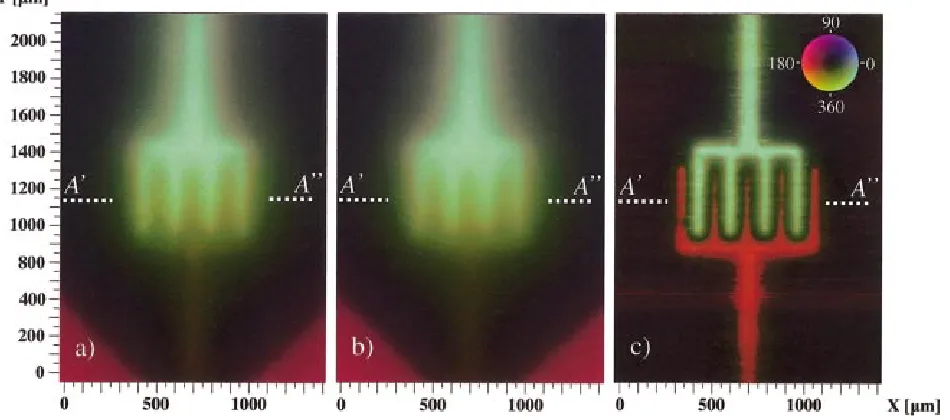
FIG. 7. 共Color兲Effect of resolution enhancement as a result of signal differences acquired for different antenna/sample separation sa. The images represent
[image:5.612.73.548.502.712.2]ered perpendicular to the surface. The dependency of the amplitude and the phase of the probe’s mechanical oscilla-tion on the probe/sample separaoscilla-tion is used to keep the sepa-ration constant in the range of several tens of nm. A quartz tuning fork, commonly used in scanning near-field optical microscopy16,17in a single oscillating arm configuration18 is utilized for probe frequency stabilization and amplitude de-tection. The technique can be employed with all types of materials used in circuit fabrication to include various met-als, dielectrics and semiconductors. After the topography ac-quisition, the probe is exchanged for the field antenna and field scanning for various separations between the antenna’s apex and the surface is performed. A static reference tip is used when the topography probe is exchanged for the an-tenna; the probes are aligned by means of an optical control using a long-focal length microscope.
IX. SCANNING RESULTS
[image:6.612.321.553.51.389.2]A surface capacitor was used to demonstrate the method described. It was fabricated by us using the standard litho-graphic process on a microwave PCB sheet as seen in the Fig. 6. The signal from the source of VNA is coupled to the port P1 of the capacitor. Port P2 is terminated by a shortcut at a distance of about 25 mm from the capacitor to allow excitation of the capacitor to higher potentials due to reso-nance in the transmission line at the frequency of interest f ⫽3.84 GHz. Both the amplitude and the phase of the signal are acquired by the antenna and stored during the scanning process.
In Figs. 7共a兲 and7共b兲 we can see field images of the normal electric field acquired for two different antenna/ sample separations; Fig. 7共c兲 shows the difference of these signals. We can clearly observe significant resolution en-hancement for the difference signal. As the antenna is sensi-tive to the field acting along the whole length of the protrud-ing conductor, the scattered field intensities at higher distances above the sample represent the main contribution to the level of acquired signal. The difference signal corre-sponds to the local electric field intensities surrounding the antenna apex only. The method also reveals the differences in the phase of electric field; these differences are indicated by different colors in the field map inserted in Fig. 7共c兲. The amplitude and the phase of electric field intensities are di-rectly determined by alternating potentials of the fingers be-longing to the two different ports P1and P2of the capacitor. The resolution enhancement is also illustrated in Fig. 8共a兲which represents cross-section A
⬘
⫺A⬙
of the signal am-plitude across the fingers of the capacitor. Figure 8共b兲 ex-poses the phase differences of about 55°. For original full-length antenna signals, the phase changes across the image are nearly indistinguishable. The increase in the phase con-trast is possible due to the fact that the difference is calcu-lated by subtracting complex amplitudes of the signals. In-deed the vector difference between two nearly identical vectors can have phase completely different from the phases of such vectors. In other words the phase contrast came from the fact that although the phase of the measured field does not change at significant heights above the surface, it doeschange for small separations above the circuit which is rep-resented by the signal difference.
The analysis of the Figs. 7 and 8 would suggest that the spatial resolution obtained by position/signal difference method is better than 30 m. This gives the ratio of the resolution to the wavelength R/ of some 3⫻10⫺4.
X. CONCLUSIONS
In order to measure electric field intensities with high resolution, a scanning setup combining topography and mi-crowave field acquisition was developed. We have presented miniaturized field probes and measurement techniques al-lowing acquisition of electric field intensity in the deep near-field region (/103⫺/104). In particular, the position/signal difference method appears to be an effective approach allow-ing one to achieve exceptional resolution with low distortion of the measured field and good quantitative field character-ization. Although we have focused our attention on acquisi-tion of the electric field components, the scanning setup and many of the described techniques may be used for magnetic field measurements utilizing a small loop antenna which would give complementary information about distribution of currents in devices under test. We believe that high resolu-tion near-field measurements can become an attractive
method for noninvasive investigation of functionality of mi-crowave devices, especially during their development and testing phase when maximum information about devices and subsystems is desired.
ACKNOWLEDGMENT
This work was supported by the Science Foundation of Ireland under Contract No. 00/PI.1/C042.
1
J. S. Dahele and A. L. Cullen, IEEE Trans. Microwave Theory Tech. 28, 752共1980兲.
2W. Spreitzer, E. Herzer, G. Fassler, and F. M. Landstorfer, Proceedings of the COST 243 Workshop, Paderborn, 1997, p. 53.
3J. Gao, A. Lauder, Q. Ren, and I. Wolf, IEEE Trans. Microwave Theory Tech. 46, 1694共1998兲.
4Y. J. Gao and I. Wolf, IEEE Trans. Microwave Theory Tech. 44, 911
共1996兲.
5V. Agrawal, P. Neuzil, and D. W. van der Weide, Appl. Phys. Lett. 71, 2343共1997兲.
6
J. D. Kraus, Antennas共McGraw–Hill, New York, 1976/1988兲, p. 389.
7T. Wei, X.-D. Xiang, W. G. Wallace-Friedman, and P. G. Schultz, Appl. Phys. Lett. 68, 3506共1996兲.
8C. C. Wei, P. K. Wei, and W. Fann, Appl. Phys. Lett. 67, 3835共1995兲. 9S. K. Dutta, C. P. Vlahacos, D. E. Steinhauer, A. S. Thanawalla, B. J.
Feenstra, F. C. Wellstood, and S. M. Anlage, Appl. Phys. Lett. 74, 1999
共1999兲.
10A. Kramer, F. Kielmann, B. Knoll, and R. Guckenberger, Micron 27, 413
共1996兲.
11A. F. Lann, M. Golosovsky, and D. Davidov, Appl. Phys. Lett. 73, 2832
共1998兲. 12
C. P. Vlahacos, D. E. Steinhauer, S. K. Dutta, B. J. Feenstra, and S. M. Angale, Appl. Phys. Lett. 72, 1778共1998兲.
13F. Duever, C. Gao, I. Takeuchi, and X.-D. Xiang, Appl. Phys. Lett. 74, 2696共1999兲.
14D. E. Steinhauer, C. P. Vlahacos, S. K. Dutta, F. C. Wellstood, and S. M. Anglage, Appl. Phys. Lett. 71, 1736共1997兲.
15
B. Knoll, F. Keilmann, A. Kramer, and R. Guckenberger, Appl. Phys. Lett.
70, 2667共1997兲.
16K. Karrai and R. D. Grober, Appl. Phys. Lett. 66, 1842共1995兲. 17D. P. Tsai and Y. L. Yuan, Appl. Phys. Lett. 73, 2724共1998兲.
18R. Kantor, M. Lesnak, N. Berdunov, and I. V. Shvets, Appl. Surf. Sci.