SWATCS65: Sentiment Classification Using an Ensemble of Class Projects
Richard Wicentowski
Swarthmore College 500 College Avenue Swarthmore, PA 19081
Abstract
This paper presents the SWATCS65 ensem-ble classifier used to identify the sentiment of tweets. The classifier was trained and tested using data provided by Semeval-2015, Task 10, subtask B with the goal to label the sen-timent of an entire tweet. The ensemble was constructed from 26 classifiers, each written by a group of one to three undergraduate stu-dents in the Fall 2014 offering of a natural lan-guage processing course at Swarthmore Col-lege. Each of the classifiers was designed in-dependently, though much of the early struc-ture was provided by in-class lab assignments. There was high variability in the final perfor-mance of each of these classifiers, which were combined using a weighted voting scheme with weights correlated with performance us-ing 5-fold cross-validation on the provided training data. The system performed very well, achieving an F1 score of 61.89.
1 Introduction
Workshops designed around competitions such as Semeval-2015 provide an excellent entry-point for undergraduate students to work on real-world prob-lems in the field by providing both the training and test data as well as a framework for comparing their work to the state-of-the-art. These competitions have a low barrier to entry while also providing students with an external motivation to continually improve their systems.
As part of the Fall 2015 offering of CPSC 065 at
Swarthmore College1, undergraduate students
en-rolled in the class were required to build a classifier for Semeval-2015 Task 10, subtask B (Rosenthal et al., 2015). The goal of this task was to provide a labeling of the sentiment expressed in a tweet: either negative, neutral or positive.
Fifty-one students were enrolled in the class and each student worked in a small group. Of the 26 groups, 23 were comprised of two students, one group had three students, and two had only one student. Approximately 35% of the students in the class (18 of 51) took this class as their first upper-level course in the discipline, having completed only the equivalents of CS1 and CS2 prior to this class.
The classifiers were developed over a seven week period beginning in the eighth week of the course.
2 Required Components
Each group was provided with boilerplate code to read in the tweets and were tasked with writing a Naive Bayes classifier to label each of the tweets. In the first two weeks, groups were required to first evaluate their system using five-fold cross-validation without any preprocessing of the tweets using only unigrams. Then they compared those results to those obtained after performing a few basic preprocessing steps (removal of stopwords, case-folding, and simple handling of negation) and
1http://goo.gl/ydgE5r
tokenization using Twokenizer (Owoputi et al., 2013).
In the third week, students read three papers from Semeval-2014 Task 9 subtask B, a similar task held in the previous year. Students were not told which papers they had to read. Each group wrote a short literature review based on their reading and implemented something they read about that sounded interesting. There was no requirement that the new piece they implemented would improve their performance, but many groups continued to add to their systems until they had made at least a minor improvement over their previous baseline.
After the third week, students were provided guidance as needed, but there were no additional re-quirements aside from writing a four-page system description paper using the conference’s style files.
3 Features
At its most basic, this sentiment classification task can be performed somewhat effectively without preprocessing the tweets, using only unigrams as features input to a supervised classifier. What sets each of the better performing classifiers apart is how the data is preprocessed, which features are extracted, whether or not external tweets or other sources (e.g. sentiment lexicons) are included, and the specifics of the classifier and its parameter settings. Many of the early modifications parroted the choices of the most successful past participants (Miura et al., 2014; Tang et al., 2014; G¨unther et al., 2014; Zhu et al., 2014).
Although there was no single modification that all teams implemented, many teams ended up with somewhat similar systems. Most teams case-folded the tweets, tokenized them using Twokenizer, then extracted only the unigrams as features. Most of the teams also included Twitter-specific preprocessing such as normalizing URLs and mentions to reduce dimensionality (e.g. nytimes.com ! someurl.net, @fmanjoo ! @someone), which has previously been shown to be effective (Amir et al., 2014).
Nearly all of the teams that attempted to handle
n-gram features
Unigrams only 18
Unigrams and bigrams 5
Unigrams, bigrams and trigrams 3 pre-processing
Case folding 24
URL normalization 22
Negation handling 22
Tokenization 21
@mention normalization 18 Stemming/lemmatization 7 Repeated character handling 7
Spell checking 6
Part-of-speech tags 3
external lexicons
Opinion lexicon (Liu et al., 2005) 14
Emoticon lists 13
Sentiment140 (Mohammad et al., 2013) 7 MPQA Subjectivity (Wilson et al., 2005) 4
classifiers
Naive Bayes 20
Support Vector Machines 10
Logistic Regression 8
Decision Lists 6
Random Forests/Boosting 2
k-Nearest Neighbors 2
[image:2.612.321.533.56.427.2]Deep belief networks 1
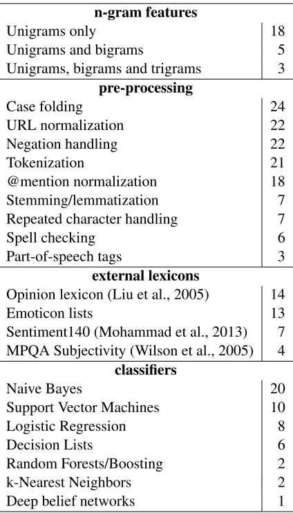
Table 1: Common features and classifiers used by the 26 systems built in the class.
negation followed the lead of (Pang et al., 2002), modifying the token in the tweet with some uniquely occurring affix such as “ NEG” to every word fol-lowing a negation word (e.g. “not”, “never”) until reaching a punctuation mark.
Although not well represented in the final sys-tems, many teams tried to use a spell checker to reduce dimensionality. After experimenting with a few options, students often chose the Jazzy2 spell
checker used by (Miura et al., 2014), though this option was largely abandoned because it produced inferior results. In particular, the dictionaries used by the spell checkers were not tailored for the colloquial, abbreviated and slangy language found
Classifier F1 score Logistic Regression 59.6 Support Vector Machines 57.4
Naive Bayes 56.5
[image:3.612.98.273.57.127.2]Decision Lists 53.5
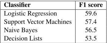
Table 2: Average F1 score for systems based on the clas-sifier used. F1 score is reported for performance on cross-validation on the training data. Note that a majority of the systems (16/26) used more than one classifier so the same system may be represented in multiple rows.
in many of the tweets, yielding high rates of false positives: words marked as incorrectly spelled that were actually spelled correctly, for example “LOL”. As an alternative to spell checking, a few teams tried to identify and correct words where the author had repeated characters for the purposes of emphasis, e.g. “sweeeeeet” or “nooooooo!”, similar to (G¨unther et al., 2014). When this occurred, teams often gave extra weight to these unigrams as a way to carry the author’s intended emphasis into the feature set.
A few students made use of a part-of-speech tagger (Owoputi et al., 2013) to include tag n-grams in the feature set, but no groups used the tags as a way to disambiguate unigram features.
Table 1 contains a summary of the most common features and classifiers used. Nine of the groups only used the Naive Bayes and decision list clas-sifiers that they had written for class assignments. The majority of the students also made extensive use of scikit-learn (Pedregosa et al., 2011), which pro-vides access to many more standard classifiers such as support vector machines, logistic regression, and k-nearest neighbors.
4 Classifiers
Students were required to implement a Naive Bayes classifier as part of the initial specification of the assignment. In a previous assignment, students had written a decision list classifier. About half of the groups (12 of 26) only used these two classifiers, ei-ther on their own or in some combination. Although a few of the better systems in the class used only
a Naive Bayes classifier, the majority of the class, and most of the best systems in the class (7 of the top 10) made use of scikit-learn (Pedregosa et al., 2011). Overall, more students tried to use SVM than Logistic Regression, perhaps because this had been talked about in class or referenced more in previous system description papers. However, similar to most of the best results from Semeval-2014, students who used the Logistic Regression classifiers tended to outperform those who used SVMs.
The large majority of the classifiers were able to read in raw tweets and produce a labeling of the test data in minutes. The small number of students who used Jazzy needed to cache the spell-checked versions of the tweets because of the very slow runtime. The deep belief network classifier was very slow, taking several hours to run.
It is difficult to make strong claims about the ef-fectiveness of each classifier given the differences in implementation between each of the systems. How-ever, as shown in Table 2, the average F1 score of systems that used Logistic Regression was higher than the average F1 score for any other classifier.
5 System Results and Combination
In consultation with the task organizers, it was agreed that rather than submitting each of the 26 systems individually, only the best-performing individual systems and a single system combining all of the systems would be submitted. As a proxy to determine how well each of the systems would do on the 2015 task, each of the 26 systems was eval-uated using five-fold cross-validation on the 2015 training data and on the test data from 2014. The three top-performing systems were submitted indi-vidually to the workshop: SWATCMW, SWATAC, and SWASH. It is likely that one or more of the next-best systems could have outperformed the systems that were submitted on the 2015 test data, but this evaluation has not been conducted. The results of each of the systems using cross-validation and on the 2014 test data are included in Table 3.
rank xvalid 2014 rank xvalid 2014 1 62.93 66.06 14 58.11 58.40 2 64.20 64.67 15 57.31 57.18 3 62.69 62.84 16 55.89 56.49 4 61.60 61.63 17 55.37 56.14 5 58.97 61.51 18 55.73 55.54 6 59.97 61.19 19 53.80 54.94 7 60.56 60.28 20 54.10 54.91 8 58.44 60.23 21 53.37 54.52 9 57.28 60.21 22 54.53 53.52 10 60.19 60.00 23 51.60 47.76 11 60.81 59.92 24 36.22 27.63 12 57.84 59.84 25 55.08 24.53 13 62.01 59.62 26 52.94 21.80
Table 3: Performance of each of the 26 systems, eval-uated using 5-fold cross-validation on the 2015 training data and sorted by their F1 score on the 2014 test data. The top three systems were submitted individually as SWATCMW, SWATAC and SWASH, respectively.
bugs in their system that caused precipitous drop-offs in performance between the cross-validation and the 2014 test data. Comparing individual system performances to those of in the 2014 task (Rosenthal et al., 2014), all of the students’ systems were in the third quartile, though some of the best of student systems were in the middle of the pack.
To obtain the final classifier, a simple weighted voting scheme was used. Each classifier was run on the test data from Semeval-2014 Task 9 subtask B. The F1 score obtained on the test data set was used as the weight for each classifier. This gave the better performing classifiers more votes in the final outcome and gave each of the students in the class a way to participate in this year’s task. Systems that had major flaws (shown as systems 24, 25 and 26 in Table 3) were omitted from the final system.
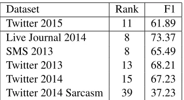
As can be seen in Table 4, the combined system did very well on the 2015 test data. On that test set, the system ranked 11th out of 40, performing quite similarly to systems ranked approximately 7 through 15.
However, looking more deeply into the progress data sets, it becomes clear that this system
strug-Dataset Rank F1
Twitter 2015 11 61.89 Live Journal 2014 8 73.37
SMS 2013 8 65.49
Twitter 2013 13 68.21 Twitter 2014 15 67.23 Twitter 2014 Sarcasm 39 37.23
Table 4: Performance of combination system compared to the 40 participants in Semeval-2015.
gled with detecting sarcasm, finishing nearly at the bottom of all the systems submitted. It is unclear why this subtlety was missed, but this was not only a problem for the combined system. Two of the three individual systems that contributed to this ensem-ble but were submitted separately to the workshop (SWATAC and SWATCMW) also did very poorly on the sarcasm subset, finishing 35th and 36th. Further analysis is warranted to see if the problem with sar-casm was widespread across all of the systems or if it was particular to the highest scoring systems whose vote was over-weighted in the final system.
6 Conclusion
We present an ensemble classifier created from 26 class projects completed during an undergraduate class in natural language processing. These projects were completed over a seven week period beginning midway through the semester. Many of the students had never taken an advanced computer science class before, but the availability of the Twitter data, pre-processing tools and machine learning toolkits made participation in this task possible even for inexperi-enced young researchers. The contributions of all of the systems yielded a highly effective sentiment classifier on all of the tweets excluding the sarcastic dataset.
7 Acknowledgements
[image:4.612.79.295.56.250.2]Flore, Shawn, Alec, Cappy, Razi, Alex, Mike S., Ruth, Lee, Elyse, A.J., Aly, Noah, Anastaisa, Ben X., David, Rita, Andrew, Peng and Chloe. Thanks!
References
Silvio Amir, Miguel B. Almeida, Bruno Martins, Jo˜ao Filgueiras, and Mario J. Silva. 2014. Tugas: Exploit-ing unlabelled data for Twitter sentiment analysis. In
Proceedings of SemEval-2014, pages 673–677. Tobias G¨unther, Jean Vancoppenolle, and Richard
Jo-hansson. 2014. RTRGO: Enhancing the GU-MLT-LT system for sentiment analysis of short messages. In
Proceedings of SemEval-2014, pages 497–502. Bing Liu, Minqing Hu, and Junsheng Cheng. 2005.
Opinion observer: analyzing and comparing opinions on the Web. InWWW’05, pages 342–351.
Yasuhide Miura, Shigeyuki Sakaki, Keigo Hattori, and Tomoko Ohkuma. 2014. TeamX: A sentiment an-alyzer with enhanced lexicon mapping and weight-ing scheme for unbalanced data. In Proceedings of SemEval-2014, pages 628–632.
Saif Mohammad, Svetlana Kiritchenko, and Xiaodan Zhu. 2013. NRC-Canada: Building the state-of-the-art in sentiment analysis of tweets. InProceedings of SemEval-2013, pages 321–327.
Olutobi Owoputi, Brendan O’Connor, Chris Dyer, Kevin Gimpel, Nathan Schneider, and Noah A. Smith. 2013. Improved part-of-speech tagging for online conver-sational text with word clusters. In Proceedings of NAACL-2013, pages 380–390.
Bo Pang, Lillian Lee, and Shivakumar Vaithyanathan. 2002. Thumbs up? sentiment classification using ma-chine learning techniques. InProceedings of EMNLP, pages 79–86.
Fabian Pedregosa, Gael Varoquaux, Alexandre Gram-fort, Vincent Michel, Bertrand Thirion, Olivier Grisel, Mathieu Blondel, Peter Prettenhofer, Ron Weiss, Vin-cent Dubourg, Jake Vanderplas, Alexandre Passos, David Cournapeau, Matthieu Brucher, Matthieu Per-rot, and Edouard Duchesnay. 2011. Scikit-learn: Ma-chine learning in Python. Journal of Machine Learn-ing Research, 12:2825–2830.
Sara Rosenthal, Alan Ritter, Preslav Nakov, and Veselin Stoyanov. 2014. Semeval-2014 task 9: Sentiment analysis in Twitter. InProceedings of SemEval-2014, pages 73–80.
Sara Rosenthal, Preslav Nakov, Svetlana Kiritchenko, Saif M Mohammad, Alan Ritter, and Veselin Stoy-anov. 2015. Semeval-2015 task 10: Sentiment analy-sis in Twitter. InProceedings Semeval-2015.
Duyu Tang, Furu Wei, Bing Qin, Ting Liu, and Ming Zhou. 2014. Coooolll: A deep learning system for
Twitter sentiment classification. In Proceedings of SemEval-2014, pages 208–212.
Theresa Wilson, Janyce Wiebe, and Paul Hoffmann. 2005. Recognizing contextual polarity in phrase-level sentiment analysis. In Proceedings of HLT/EMNLP, pages 347–354.