ETH DS3Lab at SemEval 2018 Task 7: Effectively Combining Recurrent and Convolutional Neural Networks for Relation Classification and Extraction

Proceedings of the 12th International Workshop on Semantic Evaluation (SemEval-2018), pages 689–696

ETH-DS3Lab at SemEval-2018 Task 7: Effectively Combining Recurrent

and Convolutional Neural Networks for Relation Classification and

Extraction

Jonathan Rotsztejn1_{, Nora Hollenstein}1,2_{, Ce Zhang}1 1_{Systems Group, ETH Zurich}

{rotsztej,noraho_}@ethz.ch, [email protected]

2 _{IBM Research, Zurich}

Abstract

Reliably detecting relevant relations between entities in unstructured text is a valuable re-source for knowledge extraction, which is why it has awaken significant interest in the field of Natural Language Processing. In this paper, we present a system for relation classification and extraction based on an ensemble of con-volutional and recurrent neural networks that ranked first in 3 out of the 4 subtasks at Se-mEval 2018 Task 7. We provide detailed ex-planations and grounds for the design choices behind the most relevant features and analyze their importance.

1 Introduction and related work

One of the current challenges in analyzing un-structured data is to extract valuable knowledge by detecting the relevant entities and relations be-tween them. The focus of SemEval 2018 Task 7 is on relation classification (assigning a type of

re-lation to an entity pair - Subtask 1) and relation

extraction (detecting the existence of a relation

be-tween two entities and determining its type -

Sub-task 2).

Moreover, the task distinguishes between rela-tion classificarela-tion on clean data (i.e.: manually

annotated entities - Subtask 1.1) and noisy data

(automatically annotated entities - Subtask 1.2).

It addresses semantic relations from 6 categories, all of them specific to scientific literature. Rela-tion instances are to be classified into one of the following classes: USAGE, RESULT, MODEL-FEATURE, PART-WHOLE, TOPIC, COMPARE, where the first five are asymmetrical relations and

the last is order-independent (see G´abor et al.

(2018) for a more detailed description of the task).

Since the training data was provided by the task organizers, we focused on supervised methods for relation classification and extraction. Similar sys-tems in the past have been based on Support

Vec-tor Machines (Uzuner et al.,2011;Minard et al.,

60 65 70 75 80

ICC CSD OP RS WCE EN RPE PTE CRC GD WNC

%

F1

s

co

re

Added feature

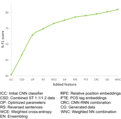
Figure 1: Feature addition study to evaluate the impact of the most relevant features on theF1score of the

5-fold cross-validated training set of Subtasks 1.1 and 1.2

2011), Na¨ıve Bayes (Zayaraz et al., 2015) and

Conditional Random Fields (Sutton and

McCal-lum,2006). More recent approaches have

experi-mented with neural network architectures (Socher

et al., 2012;Fu et al., 2017), especially

convolu-tional neural networks (CNNs) (Nguyen and

Gr-ishman,2015;Lee et al.,2017) and recurrent

neu-ral networks (RNNs) based on LSTMs (Zheng

et al., 2017;Peng et al., 2017). The system pre-sented in this article builds upon the latest im-provements in employing neural networks for re-lation classification and extraction. An overview

of the most relevant features is shown on Figure1.

2 Method

2.1 Neural architecture

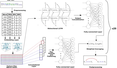
Figure2shows the full architecture of our system.

Its main component is an ensemble of CNNs and RNNs. The CNN architecture follows closely on (Kim,2014;Collobert et al.,2011). It consists of

Figure 2: Full pipeline architecture

an initial embedding layer, which is followed by a convolutional layer with multiple filter widths and feature maps with a ReLU activation func-tion, a max-pooling layer (applied over time) and a fully-connected layer, that is trained with dropout, and produces the output as logits, to which a soft-max function is applied to obtain probabilities. The RNN consists of the same initial embedding layer, followed two LSTM-based sequence

mod-els (Hochreiter and Schmidhuber, 1997), one in

the forward and one in the backward direction of the sequence, which are dynamic (i.e.: work seam-lessly for varying sequence lengths). The output and final hidden states of the forward and back-ward networks are then concatenated to a single vector. Finally, a fully-connected layer, trained with dropout, connects this vector to the logit out-puts, to which a softmax function is applied anal-ogously to obtain probabilities.

The complete architecture was replicated and

trained independently several times (see Table 2)

using different random seeds that ensured dis-tinct initial values, sample ordering, etc. in or-der to form an ensemble of classifiers, whose out-put probabilities were averaged to obtain the final probabilities for each class. We analyzed and tried several deeper and more complex neural architec-tures, such as multiple stacked LSTMs (up to 4)

and models with 2 to 4 hidden layers, but they didn’t achieve any significant improvements over the simpler models. Conclusively, the strategy that produced the best results consisted of adequately combining the individual predictions of the single

models (see section4).

2.2 Domain-specific word embeddings

We collected additional domain-specific data from scientific NLP papers to train word embeddings. All ArXiv cs.CL abstracts since 2010 (1 million

tokens) and theACL ARC corpus(90 million

to-kens; Bird et al. (2008)) were downloaded and

preprocessed. We usedgensim(ˇReh˚uˇrek and

So-jka,2010) to train word2vec embeddings on these

two data sources, and additionally the sentences provided as training data for the SemEval task (in total: 91,304,581 tokens). We experimented with embeddings of 100, 200 and 300 dimensions, where 200 dimensions yielded the best

perfor-mance for the task as shown in Figure3.

2.3 Preprocessing

Cropping sentences Since the most relevant portion of text to determine the relation type is generally the one contained between and including

the entities (Lee et al.,2017), we solely analyzed

con-40 45 50 55 60 65

Glove 50d Glove 200d NLP 100d NLP 200d NLP 300d

%

F1

s

co

re

Embedding type

Figure 3: Effect of different word embedding types based on a simple CNN classifier for Subtask 1.1

28 30 32 34 36 38 40 42 44

10 12 15 19 23

Cl

as

si

fic

at

io

n

ac

cu

ra

cy

Max. sentence length

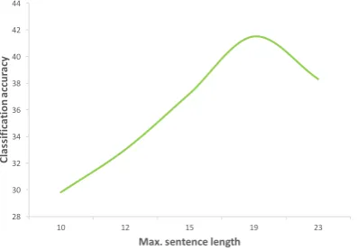
Figure 4: Effect of max. length threshold on accuracy for a preliminary RNN-based classifier

sidered every entity pair contained within a single sentence as having a potential relation. Since the probability that a relation between two entities ex-ists drops very rapidly with increasing word

dis-tance between them (see Figure5), we only

con-sidered sentences that didn’t exceed a maximum

length threshold (see Table2) between entities to

diminish the chances of predicting false positives in long sentences.

Various experiments with different thresholds between 7 and 23 words on the training set showed that the best results on sentences from scientific papers are achieved with a threshold of 19 words,

as shown in Figure4.

Cleaning sentences Some of the automatically annotated samples contained nested entities

such as <entity id=”L08-1220.16”> signal <entity

id=”L08-1220.17”>processing</entity></entity>. We

flattened these structures into simple entities and considered all the entities separately for each train and test instance. Moreover, all tokens between brackets [] and parentheses () were deleted, and

0 100 200 300 400 500 600

1 2 3 4 5 6 7 8 9 10 11 12 13 14 15 16 17 18 19 20 21 22 23 24

Sa

m

pl

es

Word distance between entities

Figure 5: Word distance between entities in a relation for training data in Subtask 1.1

<e>corpus<e>consists of independent<e>text<e>

<e>text<e>independent of consists<e>corpus<e>

<e>texts<e>from a<e>target corpus<e> Resembles

REV ERSE

Figure 6: Example of a reversed sentence

the numbers that were not part of a proper noun replaced with a single wildcard token.

Using entity tags In order to provide the neu-ral networks with explicit cues of where an entity started and ended, we used a single symbol,

rep-resented as an XML tag<e>before and after the

entity, to indicate it (Dligach et al.,2017).

Relative order strategy & number of classes

As mentioned in Section1, 5 out of the 6 relation

types are asymmetrical and the tagging is always done by using the same order for the entities as the one found in the abstracts’ text/title. For that rea-son, it was important to carefully devise a schema that allowed generalization by exploiting the infor-mation from both ordered and reversed (words that will be treated here as antonyms) relations. Apart from using the relative position embeddings

pre-sented byLee et al.(2017), for Subtask 1, we

in-corporated a full text reversal of those sentences in which a reverse relation was present, both at train-ing and testtrain-ing time. The result were instances that, although not corresponding to a valid English grammar, frequently resembled more in structure to their ordered counterparts. This has been illus-trated by an example of two instances belonging

Thus, the system could operate by using only the 6 originally specified relation types and merely learn how to identify ordered relations, rather than having to handle the two different types of pat-terns or to add extra classes to describe both the ordered and the reversed versions of each class, which helped improve the overall accuracy of the

classifier (+2.0%F1).

For Subtask 2, since no information regarding the ordering of the arguments was available (the extraction and the ordering were part of the task), we opted for a 12-class strategy: one for each of the 5 ordered and reversed relations, plus the symmetrical relation (COMPARE) and a NONE class for the negative instances, i.e.: those that didn’t contain any relation at all. An alternative 6-class approach based on presenting the sentences both ordered and reversed to the network, computing two predictions for each and afterwards consolidating both did not produce

good results (-3.4%F1).

Part-of-speech tags We used the Stanford

CoreNLP tagger (Manning et al.,2014) to obtain

POS tags for each word in every sentence in the dataset and trained high-dimensional embeddings for the 36 possible tags defined by the Penn

Tree-bank Project (Marcus et al.,1993). Moreover, the

XML tags to identify the entities and the number wildcard received their own corresponding

artifi-cial POS tag embedding (see Figure 2 for a

de-tailed example).

3 Experiments

3.1 Exploiting provided data

One of the main challenges of the task was the limited size of the training set, which is a com-mon drawback for many supervised novel ma-chine learning tasks. To overcome it, we combined

the provided datasets1 _{for Subtask 1.1 and 1.2 to}

train the models for both Subtasks (+6.2% F1).

Furthermore, we leveraged the predictions of our system for Subtasks 1.1 and 1.2 and added them

as training data for Subtask 2 (+3.6%F1).

3.2 Generating additional data

Due to the limited number of training sentences provided, we explored the following approach to augment the data: We generated automatically-tagged artificial training samples for Subtask 1 by combining the entities that appeared in the test

1_{Link to forum post 1-Link to forum post 2}

data with the text between entities and relation labels of those from the training set (see Table

1). To evaluate the quality of the sentences and

augment our data only with sensible instances, we estimated an NLP language model using the

KenLM Language Model Toolkit (Heafield,2011)

on the corpus of NLP-related text described in

Section2.2and evaluated the generated sentences

with it. Furthermore, we set a minimum thresh-old of 5 words for the length of the text between entities, limited the number of sentences gener-ated from each of them to a single instance in or-der to promote variety, and only kept those sen-tences that score a very high probability (-21 in log scale) against the language model. This process yielded 61 additional samples on the development

set (+0.7%F1).

3.3 Parameter optimization

To determine the optimal tuning for our richly pa-rameterized models, we ran a grid search over the parameter space for those parameters that were part of our automatic pipeline. The final values

and evaluated ranges are specified in Table2.

3.4 Defining the objective

The entropy loss, defined as the cross-entropy between the probability distribution out-putted by the classifier and the one implied by the correct prediction is one of the most widely used objectives for training neural networks for

classification problems (Janocha and Czarnecki,

2017). A shortcoming of this approach is that

the cross-entropy loss usually only constitutes a conveniently decomposable proxy for what the

ul-timate goal of the optimization is (Eban et al.,

2017): in this case, the macro-averagedF1 score.

Motivated by the fact that individual instances of infrequent classes have a bigger impact on the final

F1 score than those of more frequent ones (

Man-ning et al.,2008), we opted for a weighted version of the cross-entropy as loss function, where each

class had a weight w that was inversely

propor-tional to their frequency in the training set:

wclass i =

P

j#class j

Nclasses∗#class i

where#indicates the count for a certain class and

Nclassesis the total number of classes.

The weights are scaled as to preserve the expected

value of the factor ki that accompanies the

Dev set: <e>predictive performance<e>of our<e>models<e>

Train set: <e>methods<e>involve the use of probabilistic<e>generative models<e>

New sample: <e>predictive performance<e>involve the use of probabilistic<e>models<e>

Table 1: Generated sample

Parameter Final value Experiment range

Word embedding dimensionality 200 100-300

Embedding dimensionality for part-of-speech tags 30 10-50

Embedding dimensionality for relative positions 20 10-50

Number of CNN filters 192 64-384

Sizes of CNN filters 2 to 7 2-4 to 5-9

Norm regularization parameter (λ) 0.01 0.0-1.0

Number of LSTM units (RNN) 600 0-2400

Dropout probability (CNN and RNN) 0.5 0.0-0.7

Initial learning rate 0.01 0.001-0.1

Number of epochs (Subtask 1) 200 20-400

Number of epochs (Subtask 2) 10 5-40

Ensemble size 20 1-30

Training batch size 64 32-192

Upsampling ratio (only Subtask 2) 1.0 0.0-5.0

Max. sentence length (only subtask 2) 19 7-23

Table 2: Final parameter values and their explored ranges

TOPIC-R RESULT-R COMPARE RESULT MODEL-FEAT-R PART-WHOLE-R TOPIC PART-WHOLE USAGE-R MODEL-FEAT USAGE NONE

619 349

334 275 238 155 152 137 136 58 23

34,824

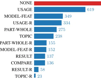
Figure 7: Class frequencies for Subtask 2

formula: L = ₋Pkilog(yi), which is equal to

wy_i0 for the weighted cross-entropy andy0_i for the

unweighted version, wherey0_i = 1for the correct

class and yi is the predicted probability for that

class. Illustrating this concept, it can be observed

that a single instance of classTOPIC (support of

only 6 instances) could account for up to 2.8% of the final score on the test set. This function proved to be a better surrogate for the global final score

than the standard cross-entropy (+1.6%F1).

3.5 Upsampling

One of the challenges of our approach for Subtask 2 was the existence of a large imbalance between the target classes. Namely, the NONE class

con-stituted the clear majority (Figure7). To overcome

it, we resorted to an upsampling scheme for which we defined an arbitrary ratio of positive to neg-ative examples to present to the networks for the

combination of all positive classes (+12.2%F1).

4 Training and validating the model The neural networks were trained using an Adam

optimizer with parameter valuesβ2 = 0.9, β2 =

0.999, = 1e₋08 (suggested default values in

the TensorFlow library (Abadi et al.,2015)) with a

step learning rate decay scheme on top of it. This consisted in halving the learning rate every 25 and 1 iterations through the whole dataset for Subtasks 1 and 2 respectively (note: the size of the upsam-pled dataset for Subtask 2 was about 25 times that of Subtask 1), starting from the initial value

deter-mined in Section3.3. In order to avoid overfitting

Combining predictions During the

develop-ment, we observed that similar F1 scores could

be achieved by using either a convolutional neu-ral network or a recurrent one separately, but the combination of both outperformed the individual models. Moreover, since the RNN-based architec-ture had a tendency to obtain better results than its CNN-based counterpart for long sequences, we combined both predictions in such a way that a higher weight was assigned to the RNN predic-tions for longer sentences by applying:

wrnn,i= 0.5 +sign(si)·s2i, where

si=

lengthi−minj(lengthj)

maxj(lengthj)−minj(lengthj) −

0.5

andlengthiis the length of the i-th sentence.

Post-processing To enforce consistency with the text annotation scheme, some rules that were not built into the system had to be applied ex-post. First, predictions of reversed relations should not be of type COMPARE, since it is the only symmet-rical relation. When this condition occurred, we simply predicted the class that had the 2nd high-est probability. Second, each entity could only be part of one relation. To address this for Subtask 2, we run a conflict-solving algorithm that, in case of overlaps, always preferred short relations (cf.

Fig-ure3]) and broke ties by choosing the relation with

the most frequent class in the training data and at random when it persisted.

5 Results

5.1 Feature analysis

We conducted a feature addition study to evalu-ate the impact of the most relevant features on

the F1 score of the 5-fold cross-validated

train-ing/development set of Subtasks 1.1 and 1.2. The results have been previously shown in

Fig-ure1. It can be observed from the plot that

sub-stantial gains can be obtained by applying stan-dalone data manipulation techniques that are in-dependent of the type of classifier used, such as

combining the data of subtask 1.1 and 1.2 (CSD

in Figure1), reversing the sentences (RS),

gener-ating additional data (GD) and the pre-processing

techniques from Section2.3. Moreover, as in most

machine learning problems, appropriately tuning the model hyperparameters also has a significant impact on the final score.

Subtask P R F1

1.1 79.2 84.4 81.7 1.2 93.3 87.7 90.4 2.E 40.9 55.3 48.8 2.C 41.9 60.0 49.3

Table 3: Precision (P), recall (R) andF1-score (F1) in

% on the test set by Subtask

Relation type P R F1

COMPARE 100.00 95.24 97.56 MODEL-FEATURE 71.01 74.24 72.59 PART-WHOLE 78.87 80.00 79.43

RESULT 87.50 70.00 77.78

TOPIC 50.00 100.00 66.67

USAGE 87.86 86.86 87.36

Micro-averaged total 82.82 82.82 82.82 Macro-averaged total 79.21 84.39 81.72 Table 4: Detailed results (Precision (P), recall (R) and

F1-score (F1)) in % for each relation type on the test set

for Subtask 1.1

5.2 Final results

After presenting and analyzing the impact of each system feature separately, we show the overall re-sults in this section. The final rere-sults on the

offi-cial test set are presented on Table3, ranking 1st

in Subtasks 1.1, 1.2 and Subtask 2.C (joint result of classification and extraction) and 2nd for 2.E

(relation extraction only). Furthermore, Table 4

shows the differences in performance between re-lation types for Subtask 1.1.

6 Conclusion

References

Mart´ın Abadi, Ashish Agarwal, et al. 2015. Ten-sorFlow: Large-scale machine learning on hetero-geneous systems. Software available from tensor-flow.org.

Steven Bird, Robert Dale, Bonnie J Dorr, Bryan Gib-son, Mark Thomas Joseph, Min-Yen Kan, Dongwon Lee, Brett Powley, Dragomir R Radev, and Yee Fan Tan. 2008. The ACL anthology reference corpus: A reference dataset for bibliographic research in com-putational linguistics. EUROPEAN LANGUAGE RESOURCES ASSOC-ELRA.

Ronan Collobert, Jason Weston, L´eon Bottou, Michael Karlen, Koray Kavukcuoglu, and Pavel Kuksa. 2011. Natural language processing (almost) from scratch. Journal of Machine Learning Research, 12(Aug):2493–2537.

Dmitriy Dligach, Timothy Miller, Chen Lin, Steven Bethard, and Guergana Savova. 2017. Neural tem-poral relation extraction. EACL 2017, page 746. Elad Eban, Mariano Schain, Alan Mackey, Ariel

Gor-don, Ryan Rifkin, and Gal Elidan. 2017. Scalable learning of non-decomposable objectives. In Artifi-cial Intelligence and Statistics, pages 832–840. Lisheng Fu, Thien Huu Nguyen, Bonan Min, and

Ralph Grishman. 2017. Domain adaptation for re-lation extraction with domain adversarial neural net-work. In Proceedings of the Eighth International Joint Conference on Natural Language Processing (Volume 2: Short Papers), volume 2, pages 425–429. Kata G´abor, Davide Buscaldi, Anne-Kathrin Schu-mann, Behrang QasemiZadeh, Hafa Zargayouna, and Thierry Charnois. 2018. SemEval-2018 Task 7: Semantic Relation Extraction and Classifica-tion in Scientific Papers. In Proceedings of the 12th International Workshop on Semantic Evalua-tion (SemEval-2018).

Kenneth Heafield. 2011. Kenlm: Faster and smaller language model queries. InProceedings of the Sixth Workshop on Statistical Machine Translation, pages 187–197. Association for Computational Linguis-tics.

Sepp Hochreiter and J¨urgen Schmidhuber. 1997. Long short-term memory. Neural computation, 9(8):1735–1780.

Katarzyna Janocha and Wojciech Marian Czarnecki. 2017. On loss functions for deep neural networks in classification. arXiv preprint arXiv:1702.05659. Yoon Kim. 2014. Convolutional neural

net-works for sentence classification. arXiv preprint arXiv:1408.5882.

Ji Young Lee, Franck Dernoncourt, and Peter Szolovits. 2017. MIT at SemEval-2017 Task 10: Relation Extraction with Convolutional Neural Net-works. arXiv preprint arXiv:1704.01523.

Christopher D Manning, Prabhakar Raghavan, Hinrich Sch¨utze, et al. 2008. Introduction to information re-trieval, volume 1. Cambridge university press Cam-bridge.

Christopher D. Manning, Mihai Surdeanu, John Bauer, Jenny Finkel, Steven J. Bethard, and David Mc-Closky. 2014. The Stanford CoreNLP natural lan-guage processing toolkit. InAssociation for Compu-tational Linguistics (ACL) System Demonstrations, pages 55–60.

Mitchell P Marcus, Mary Ann Marcinkiewicz, and Beatrice Santorini. 1993. Building a large annotated corpus of English: The Penn Treebank. Computa-tional linguistics, 19(2):313–330.

Anne-Lyse Minard, Anne-Laure Ligozat, and Brigitte Grau. 2011. Multi-class SVM for relation extrac-tion from clinical reports. InProceedings of the In-ternational Conference Recent Advances in Natural Language Processing 2011, pages 604–609.

Thien Huu Nguyen and Ralph Grishman. 2015. Rela-tion extracRela-tion: Perspective from convoluRela-tional neu-ral networks. InProceedings of the 1st Workshop on Vector Space Modeling for Natural Language Pro-cessing, pages 39–48.

Nanyun Peng, Hoifung Poon, Chris Quirk, Kristina Toutanova, and Wen-tau Yih. 2017. Cross-sentence n-ary relation extraction with graph LSTMs. arXiv preprint arXiv:1708.03743.

Radim ˇReh˚uˇrek and Petr Sojka. 2010. Software Frame-work for Topic Modelling with Large Corpora. In Proceedings of the LREC 2010 Workshop on New Challenges for NLP Frameworks, pages 45–50, Val-letta, Malta. ELRA. http://is.muni.cz/ publication/884893/en.

Richard Socher, Brody Huval, Christopher D Manning, and Andrew Y Ng. 2012. Semantic compositional-ity through recursive matrix-vector spaces. In Pro-ceedings of the 2012 joint conference on empirical methods in natural language processing and com-putational natural language learning, pages 1201– 1211. Association for Computational Linguistics.

Charles Sutton and Andrew McCallum. 2006. An introduction to conditional random fields for rela-tional learning, volume 2. Introduction to statistical relational learning. MIT Press.

¨Ozlem Uzuner, Brett R South, Shuying Shen, and Scott L DuVall. 2011. 2010 i2b2/va challenge on concepts, assertions, and relations in clinical text. Journal of the American Medical Informatics Asso-ciation, 18(5):552–556.