1
ECE-320: Linear Control Systems
Homework 2
Due: Friday March 20, 2015 at the beginning of class
1)(Model Matching) Consider the following closed loop system, with plant and controller .
One way to choose the controller is to try and make your closed loop system match a transfer function that you choose (hence the name model matching). Let’s assume that our desired closed loop transfer function, , our plant can be written in terms of numerators and denominators as
Show that our controller is then
Note that there are some restrictions here, in that for implementation purposes the controller must be stable, and it must be proper.
2) For the following system, with plant , and controller
a) Using the results from problem 1, determine the controller so that the closed loop system matches a second order ITAE (Integral of Time and Absolute Error) optimal system, i.e., so that the closed loop transfer function is
Anwes. , note that there is a pole/zero cancellation between the controller and the plant and
there is a pole at zero in the controller.
b) Show that the damping ratio for this system is 0.7, the closed loop poles of this system are at . For faster response should be large or small?
c) Determine the controller so that the closed loop system matches a third order deadbeat system, i.e., so that the closed loop transfer function is
Ans. , note that there is a pole/zero cancellation between the controller and the
plant and there is a pole at zero in the controller.
( )
p
G s G sc( )
( ) o G s ( ) ( ) ( ) ( ) ( ) ( ) p o o p o p N s N s
s G s
s G
D s D
( ) ( ) ( ) ( ) ( ) ( ) p o o c o pN s D s G s
N s D s N s
1 ( ) 1 p G s s
G sc( )
2 0
0 2 2
0 0 ( ) 1.4 G s s s 2 0 0 ( 1) ( )
( 1.4 )
c s G s s s 0 0
0.7 j0.714
0
3 0
0 3 2 2 3
0 0 0
( )
1.90 2.20
G s
s s s
3 0 2 2 0 0 ( 1) ( )
( 1.9 2.20 )
c
s G s
s s s
2
3) Consider the following simple feedback control block diagram. The plant is . The input is a unit
step.
a) Determine the settling time and steady state error of the plant alone (assuming there is no feedback)
b) Assuming a proportional controller, , determine the closed loop transfer function,
c) Assuming a proportional controller, , determine the value of so the steady state error for a unit step is 0.1, and the corresponding settling time for the system.
d) Assuming a proportional controller, ,determine the value of so the settling time is 0.5 seconds, and the corresponding steady state error.
e) Assuming an integral controller, , determine closed loop transfer function,
f) Assuming an integral controller, , determine the value of so the steady state error for a unit step is less than 0.1 and the system is stable.
Partial Answers:
4) Consider the following simple feedback control block diagram. The plant is .
a) What is the bandwidth of the plant alone (assuming there is no feedback)
b) Assuming a proportional controller, , determine the closed loop transfer function,
c) Assuming a proportional controller, , determine the value of so the bandwidth of the closed loop
system is 27 rad/sec.
d) Assuming the proportional controller from problem c, determine the settling time and the steady state error for a unit step.
Partial Answers: 7, 5, 7/27, 4/27
5) An ideal second order system has the transfer function
G s
o( )
. The system specifications for a step input are asfollows:
Percent Overshoot < 5%, Settling Time < 4 seconds (2% criteria), Peak Time < 1 second
Sketch, in the complex plane, the permissible area for the poles of
G s
o( )
in order to achieve the desired response. ( )4 2
p G s
s
( )
c p
G s k G s0( )
( )
c p
G s k kp
( )
c p
G s k kp
( ) /
c i
G s k s G s0( )
( ) /
c i
G s k s ki
1, 0.5, 18, 2, 0.1, 0.5, 0
s ess p kp Ts ess i
T k k
( )
7 4
p
G s s
( )
c p
G s k G s0( )
( )
c p
3
6) For systems with the following transfer functions:
1 6
( ) ( )
2 ( 2)( 3)
a b
H s H s s
s s s
a) Determine the unit step and unit ramp response for each system using Laplace transforms. Your answer should be time domain functions ya (t) and yb (t) .
b) From these time domain functions, determine the steady state errors for a unit step and unit ramp input.
The following Matlab code can be used to estimate the step and ramp response for 5 seconds for transfer function Hb (s) .
H = tf([1 6],[1 5 6]); % enter the transfer function
t = [0:0.01:5]; % t goes from 0 to 5 by increments of 0.01 ustep = ones(1,length(t)); % the step input is all ones, u(t) = 1;
uramp = t; % the ramp input is has the input u(t) = t;
ystep = lsim(H,ustep,t); % find the step response yramp = lsim(H,uramp,t); % find the ramp response
figure; % make a new figure
orient tall % or orient landscape, use more of the page
subplot(2,1,1); % put two graphs on one piece of paper plot(t,ustep,'.-',t,ystep,'-'); % plot input/output with different line types
grid; % put a grid on the graph
legend('Step Input','Step Response',4); % put a legend on the graph
subplot(2,1,2); % second of two graphs on one piece of paper plot(t,uramp,'.-',t,yramp,'-'); % plot input/output with different line types
grid; % put a grid on the graph
legend('Ramp Input','Ramp Response',4); % put a legend on the graph
c) Plot the step and ramp response for both systems (a and b) and indicate the steady state errors on the graph. Draw on the graph to show you know what the steady state errors are.
Ans. Steady state errors for a unit step input: 0.5,0; for a unit ramp input : infinity and 0.666
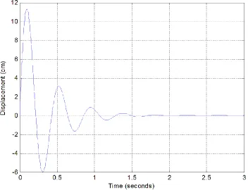
7) The differential equation model of an ideal second order system is
2 2
( ) 2
n( )
n( )
= K
n(
)
y t
y t
y t
x t
Here Kis the static gain,
nis the natural frequency, and is the damping ratio. These are the parameters we need to determine for these models.You will need to download and uncompress the file Homework2 Files.rar. The Matlab file
4
the time, input, and output values for the system. After this, you are to modify your guesses for the damping ratio, the natural frequency, and the static gain. The Matlab script second_order_driver.m then runs the Simulink model file Second_Order_System.mdl and plots the results of your model with the measured data.
You are to change the parameters in the Matlab driver file to try and get your model to match the step response of the unknown system as well as possible. Once you are done, save the graph with the step responses of the two systems and put it in your memo.
You will need to do this for the data files measured_1, measured_2, measured_3, and measured_4.
Your homework should contain four figures for this problem.
8) One of the methods that can be used to identify and
nfor mechanical systems the log-decrement method, which we will derive in this problem. If our system is at rest and we provide the mass with an initial displacement away from equilibrium, the response due to this displacement can be written1
( )
cos(
)
ntd
x t
Ae
t
where
1
( )
x t
= displacement of the mass as a function of time = damping ratio
n
= natural frequencyd
= damped frequency = 2 1n
After the mass is released, the mass will oscillate back and forth with period given by d 2 d
T
, so if we measure
the period of the oscillation (
T
d) we can estimate
d.Let's assumet
0is the time of one peak of the cosine. Sincethe cosine is periodic, subsequent peaks will occur at times given by
t
n
t
0nT
d, wheren
is an integer.a) Show that 1 0
1 ( ) ( )
n dT n
n
x t e x t
b) If we define the log decrement as 1 0 1
( ) ln
( )n x t x t
show that we can compute the damping ratio as
2 2 2 4n
5
Figure 1. Initial condition response for second order system A.
[image:5.612.127.479.374.644.2]6
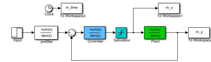
9) (Matlab/Simulink) Download and uncompress the file Model_Matching.rar from the class website. The
[image:6.612.73.520.82.215.2]file closedloop.slx is a Simulink file the for a simple closed loop system, as shown below in in Figure 3.
Figure 3. Simple feedback control system
In this system the plant is the thing we want to control, the controller modifies the behavior of the plant, and we have included a limit on the control effort (the Saturation block). Many real systems have limits on the control effort, as you will see.
The file closedloop_driver.m is the Matlab driver file that loads parameters and transfer functions into the Matlab workspace for the Simulink file to use. Using these two programs we can look at some model matching systems and some examples of what happens when the model does not match the real system. Also this gives us a review of Matlab and Simulink.
If you run the programs as they are you should get a response like that shown in Figure 4 on the next page. This figure shows the response to the plant (the thing we want to control) in the top graph. The middle graph shows a control system using model matching for a 1 cm input. In this graph the red line shows the response of the closed loop transfer function we expect to get if the mathematical model of the plant is exact, and the red line shows the results using the model matching control system. You should note that the control system has a faster response, smaller overshoot, and a steady state error of zero (the output is equal to the input in steady state). The last graph shows the control effort of the system. Most practical systems have a limit on the allowed control effort since real systems (like op amps) tend to saturate.
a) Modify the parameter
0to get the fastest response you can without saturating the control effort (the controleffort should remain below 2). Note that the control effort is maximum at the beginning and then dies down, this is common for controllers. At this point our model of the plant and the true plant have the transfer
function
2 100 ( )
2 10
p s
s G
s
.Turn in your graph.
In the next few parts we will look at examples when the model is not matched exactly. For each of these parts
use the value of
0you determined in part a.b) Assume the true plant has the transfer function
2 20 ( )
20
p s
s G
s
7
c) Assume the true plant has the transfer function
2
25 50
( )
20
p
G s s
s s
. Rerun the simulation and turn in your results.
d) Assume the true plant has the transfer function
3 2 ( )
0.1 2
1 0
0 0
p s
s s
G
s
. Rerun the simulation and turn in your results.
e) Assume the true plant has the transfer function
2 100 ( )
20 2
p s
s G
s
. Set the final time to 3.5 seconds (Tf = 3.5) and rerun the simulation and turn in your results. What happens in this case?
Figure 4. Response of a plant and an ITAE closedloop model matching system.
0 0.5 1 1.5 2 2.5
0 2 4 6 8 10 12 14
Time (sec)
y
(
c
m
)
Open Loop Plant
0 0.5 1 1.5 2 2.5
0 0.5 1 1.5
Time (sec)
y
(
c
m
)
Closedloop Model Matching, 0 = 5rad/sec
Model Matching Model
0 0.5 1 1.5 2 2.5
-2 -1 0 1 2
Control Effort
Time (sec)
u
(
c
m