Bob Throne

ECE-205

Dynamical

Systems

Course Notes

Fall 2010

1.0 Electrical Systems

The types of dynamical systems we will be studying can be modeled in terms of algebraic equations, differential equations, or integral equations. We will begin by looking at familiar mathematical models of ideal resistors, ideal capacitors, and ideal inductors. Then we will begin putting these models together to develop models for RL and RC circuits. Finally, we will review solution techniques for the first order differential equation we derive to model the systems.

1.1 Ideal Resistors

The governing equation for a resistor with resistanceR is given by Ohm’s law,

( ) ( )

v t =Ri t

where v t( ) is the voltage across the resistor and i t( ) is the current through the resistor. HereRis

measured in Ohms, is measured in volts, and is measured in amps. The entire expression must be in volts, so we get the unit expression

( )

v t i t( )

[volts] = [Ohms][amps] 1.2 Ideal Capacitors

The governing equation for a capacitor with capacitance C is given by

( )

( ) dv t

i t C dt

=

HereCis measured in farads, and again is measured in volts and is measured in amps. This expression also helps us with the units. The entire expression must be in terms of current , so looking at the differential relationship we can determine the unit expression

( )

v t i t( )

[amps] = [farads][volts]/[seconds]

We can integrate this equation from an initial time t₀ up to the current time t as follows:

( )

( ) dv t

i t C dt

=

1

( ) ( )

i t dt dv t

C =

Next, since we want to integrate up to a final time , we need to use a dummy variable in the integral that is not t. This is an important habit to get into—do not use t as the dummy variable of integration if we expect a function of time as the output! Here we have chosen to use the dummy variable

t

0

)

) (

(

1

( ) ( )

o v t t

t v t

i d dv

C

∫

∫

Carrying out the integration we get

0

0

1

)

( ) ( ) (

t

t

i d v t v t

C

∫

which we can rearrange as

0

0

1 )

( ) ( ( )

t

t

v t v t i

C λ λd

+

=

∫

This expression tells us there are two components to the voltage across a capacitor, the initial voltage and the part due to any current flowing through the capacitor after that time,

0

( )

v t

0 1

( )

t

t

i d

C

∫

Finally, these expressions help us determine some important characteristics of our ideal capacitor: • If the voltage across the capacitor is constant, then the current through the capacitor must be zero

since the current is proportional to the rate of change of the voltage. Hence, a capacitor is an open circuit to dc.

• It is not possible to change the voltage across a capacitor in zero time .The voltage across a capacitor must be a continuous function of time, otherwise an infinite amount of current would be required.

1.3 Ideal Inductors

The governing equation for an inductor with inductance L is given by

( )

( ) di t

v t L dt

=

HereL is measured in henrys, and again is measured in volts and is measured in amps. This expression also helps us with the units. The entire expression must be in terms of voltage , so looking at the differential relationship we can determine the unit expression

( )

v t i t( )

[volts] = [henrys][amps]/[seconds]

We can integrate this equation from an initial time t₀ up to the current time t as follows:

( )

( ) di t

v t L dt

=

1

( ) ( )

v t dt di t

Next, since we want to integrate up to a final time , so we again have chosen to use the dummy variable

t

λ. Also we incorporate the fact that at time the current is, while at time the current is .

0

t i t( )₀ t

( )

i t

0

)

) (

(

1

( ) ( )

o i t t

t i t

v d di

L

∫

∫

Carrying out the integration we get

0

0

1

)

( ) ( ) (

t

t

v d i t i t

L

∫

which we can rearrange as

0

0

1 )

( ) ( ( )

t

t

i t i t v

L λ λd

+

=

∫

This expression tells us there are two components to the current through an inductor, the initial current and the part due to any voltage across the inductor after that time,

0

( )

i t

0 1

( )

t

t

v d

L

∫

Finally, these expressions help us determine some important characteristics of our ideal inductor: • If the current thought an inductor is constant, then the voltage across the inductor must be zero

since the voltage is proportional to the rate of change of the current. Hence, an inductor is a short circuit to dc.

2.0 First Order Circuits

A first order circuit is a circuit with one effective energy storage element, either an inductor or a capacitor. (In some circuits it may be possible to combine multiple capacitors or inductors into one equivalent capacitor or inductor.) We begin this section with the derivation of the governing differential equation for various first order circuits. We will then put the first order equation into a standard form that allows us to easily determine physical characteristics of the circuit. Next we show an alternative method for checking some parts of the governing differential equations. We then solve the differential equations for the case of piecewise constant inputs, and finish the section with an alternative method of solving the differential equations using integrating factors.

2.1 Governing Differential Equations for First Order Circuits

In this section we derive the governing differential equations that model various RL and RC circuits. We then put the governing first order differential equations into a standard form, which allows us to read off descriptive information about the system very easily. The standard form we will use is

( )

( ) ( )

dy t

y t Kx t dt

τ + =

Here we assume the system input isx t( ) and the system output isy t( ). τ is the system time constant, which indicates how long it will take the system to reach steady state for a step (constant) input. K is the static gain of the system. For a constant input of amplitudeA (x t( )= Au t( ), where is the unit step function), in steady state we have

( )

u t

( ) 0

dy t

dt = and y t( )=Kx( )t =KA. Hence the static gain lets us easily compute the steady state value of the output. For circuits with capacitors the differential equation will in general be in terms of a voltage (the output will be a voltage), while for circuits with

inductors the differential equation will in general be in terms of current (the output will be a current) .

( )

y t

(

y t)

Example 2.1.1. Consider the RC circuit shown in Figure 2.1. The voltage source is . We start to derive the governing differential equation by determining the single current in the loop

( )

s v t

( ) ( ) ( )

( ) s c ( ) c

R C

v d

i i v

R

t v t t

t − t C

dt

= = =

or

( ) ( ) ( )

c t s c

dv v

C dt

v R t − t

=

where is the voltage across the capacitor and the current in the loop is equal to the current through the resistor and the current through the capacitor . We can put this into a more standard form by rearranging the terms

( )

c v t

( )

R

i t i t_C( )

( )

( ) ( )

c

c s

dv

( ) ( ) ( ) c c s dv v t

t v t dt

τ + =

Here the static gainK =1.

R

( )

s

v t

( )

c

v t

-+

+

-

C

Figure 2.1. Circuit for Example 2.1.1.

Example 2.1.2. Consider the RC circuit shown in Figure 2.2. Again the voltage source is . We again start to derive the governing differential equation by determining the current through resistor

( ) s v t a R , ( )

( ) s c( )

a

v

i t v

R t − t

=

This current must be equal to the sum of the currents through the capacitor and R_b,

(

( ) c ) ( )

b c v dv i C d t R t t

t = +

Equating these we get the governing differential equation:

( ) ( ) ( ) (

( ) s c c c )

a b

v v

i t C

R t v d t dv R t t t = − = +

Rearranging terms we get

1 1

( ) 1

( ) ( ) c s a b c a dv C v

dt R R R

t

t t

⎛ ⎞

+_⎜ + _⎟

⎝ ⎠ = v

1 ( ) ( ) ( ) a b s a b c c a t R t dv R C v

dt + R R R v t

+

=

or

( )

( ) ( )

a b b

s a b c a b c R dv v v R d

R C t t

R

t t

R + = R

With time constant a b

a b

R C R R R

τ =

+ and static gain

b

a b

R K

R +R

= we get

( )

( ) ( )

c

c s

t dv

v v

dt t K t

τ + =

R

R

( )

s

v t

v t

c

( )

-+ +

-

C

Figure 2.2. Circuit used in Example 2.1.2.

Example 2.1.3. Consider the operational-amplifier circuit shown in Figure 2.3. The input voltage is againv t_s( ) and the output voltage (the voltage across the load resistorR_L) is the same as the voltage across the capacitor (since the + terminal of the op amp is assumed to be grounded). We will assume an ideal op amp, which implies the conditions

( ) ( ) 0 ( ) ( )

i t i t

v t v t

+ −

+ −

= =

=

Let’s look at the currents flowing into the negative (feedback) terminal of the amp using the ideal op-amp model. Since for our exop-ample the non-inverting terminal is tied to ground we have v t+( )=0. With these assumptions our governing differential equation becomes

( ) ( ) ( )

0 s c c

a b

v t v t dv t C

R R d

= + +

t Rearranging this gives

( ) ( ) _s( )

b a

c c

dv t v t v t C

dt + R = − R or

( )

( ) b ( )

b s

c c

a

dv t R

R C v t v

dt + = −R t Setting the time constant τ =R C_b and static gain b

a

R K

R

( )

( ) ( )

c

c s

dv t

v t Kv t dt

τ + =

R

C

Figure 2.3. Circuit for Example 2.1.3.

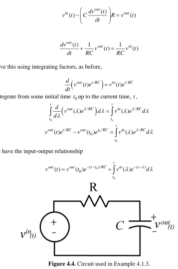
Example 2.1.4. Consider the RL circuit shown in Figure 2.4. The single current in the loop is given by

( ) ( )

( ) v ts v tL

i t

R

− =

where

(

( ) )

L

d L i t v

t t

d

=

Combining and rearranging we get

( ) ( )

( ) s

di t

L Ri t v

dt + = t or

( ) 1

( ) _s( )

L di t

i t v R dt + = R t With time constant L

R

τ = and static gain K 1 R

= the governing differential equation is

( )

( ) s( )

di t

i t Kv

dt t

τ + =

R

( )

c

v t

- +

R

+

-+

-( )

s

R

+

( )

L

v t

( )

s

v t

L

-Figure 2.4. Circuit for Example 2.1.4.

Example 2.1.5. Consider the RC circuit shown in Figure 2.5. The single current source must be divided between the current flowing through resistor R_b and the current flowing through the capacitorC,

( ) ( )

( ) c c

s

b

v dv

i t C

R t

t t

d

= +

Rearranging we get

( )

( ) ( )

c

b c

dv

RC t v t R dt + = b si t

With time constantτ =R_bC and static gain K =R_b the governing differential equation is

( )

( ) ( )

c

c s

t dv

v

dt t Ki t

τ + =

R

( )

c

v t

+

R

( )

s

i t

C

2.2 Thevenin Resistance, Time Constants, and Static Gain

Although we are focusing our attention on deriving the governing equations for first order circuits, it is useful and very convenient to be able to check our equations as much as possible.

First of all, for first order RC circuits the time constants will be of the formτ =R C_{th eq} whereR_th is the Thevenin resistance seen from the ports of the equivalent capacitor, . For first order RL circuits the time constants will be of the form

eq

C

eq th L R

τ = whereR_th is the Thevenin resistance seen from the ports of the equivalent inductor, L_eq. Recall that when determining the Thevenin resistance all independent voltage sources are treated as short circuits, and all independent current sources are treated as open circuits.

Secondly, if we are looking at constant inputs, then we use the fact that a capacitor is an open circuit to dc and an inductor is a short circuit to dc. In addition, for constant inputs in steady state all of the time derivatives are zero (in steady state nothing changes in time).

Example 2.2.1. Consider the circuit shown in Figure 2.1 (Example 2.1.1). The Thevenin resistance seen from the capacitor is equal toR, so the time constant is τ =RC. For a dc input, the capacitor looks like an open circuit, so in steady state the voltage across the capacitor is equal to v_s, the input voltage, so the static gain is K =1. These results match our previous results.

Example 2.2.2. Consider the circuit shown in Figure 2.2 (Example 2.1.2). The Thevenin resistance seen from the capacitor is || a b

th a b

a b

R R R R

R R

R

= =

+ , so the time constant is

a b th

a b

R R R

C R C

R

τ = =

+ . For a dc input,

the capacitor looks like an open circuit, so in steady state the voltage across the capacitor is given by the voltage divider relationship b

c

a b

R v

R R

=

+ vs, so the static gain is

b

a b

R K

R +R

= . These results match our previous results.

Example 2.2.3. Consider the circuit shown in Figure 2.3 (Example 2.1.3). The Thevenin resistance seen by the capacitor is a little more difficult to determine, and to do it correctly is beyond the scope of this course. For a dc input, the capacitor looks like an open circuit, so summing the currents into the negative terminal of the op amp we have c s 0

b a

v v

R + R = , or in steady state

b

c s

a

R v

R

= − v Hence the static gain is

b a

R K

R

= − .

Example 2.2.4. Consider the circuit shown in Figure 2.4 (Example 2.1.4). The Thevenin resistance seen by the inductor is R_th =R. For a dc input, the inductor looks like a short circuit. Hence the steady state current flowing in the circuit for a dc input is i 1 v_s

R

= , so the static gain is K 1 R

Example 2.2.5. Consider the circuit shown in Figure 2.5 (Example 2.1.5). The Thevenin resistance seen by the capacitor is R_th =R_b so the time constant is τ =R C_b . For a dc input the capacitor looks like an open circuit, so in steady state v_c =R_bi, so the static gain is K =R_b.

2.3 Solving First Order Differential Equations

In this section we will go over two methods for solving first order differential equations. We will initially solve the equations by breaking the solution into the natural response (the response with no input) and then the forced response (the response when the input is turned on). We will apply this method to problems where the input is a constant value, or is switched between constant values. This method will also work with any input, and we will examine the results for a sinusoidal input later. In the last section we will go over a different method of solution using integrating factors, which will work for any type of input, and is an important method in helping us characterize how a system will respond to any type of input.

2.3.1 Solution using Natural and Forced Responses

Consider a system described by the first order differential equation

( )

( ) ( )

dy t

y t Kx t dt

τ + =

In this equation, τ is the time constant and K is the static gain. We will solve this equation in two parts. We will first determine the natural response, ( . The natural response is the when the input is zero. Then we will determine the forced response, . The forced response is the response due to the input only. The total response is then the sum of the natural and forced responses, .

)

n y t

( ) f

y t

( ) _n( ) _f( )

y t =y t +y t

Natural Response: To determine the natural response we assume there is no input in the system, so we have the equation

( )

( ) 0

n

n

dy t

y t dt

τ + =

Let’s assume a solution of the form , wherec and are parameters to be determined. Substituting this assumption into the differential equation we get

( ) rt

n

y t =c e r

[ 1]

rt rt rt

rce ce ce r

τ + = τ + =0

Ifc=0 then we are done, and the natural response will bey t_n( )=0. This solution certainly satisfies the differential equation. However, ifc≠0, and since rt can never be zero, we must have

e τr+ =1 0, or

1

r

τ

= − . In this case the natural response will be

/

( ) t

n

y t =ce− τ.

0 0 ( )

0

t x t

A t

< ≥ ⎧ = ⎨ ⎩ Then for t≥0 we have the equation

( )

( )

f

f dy t

y t K

dt

τ + = A

Since this is a linear ordinary differential equation we only need to find one solution. One obvious solution to this equation is the solution in steady state, when dy tf( ) 0

dt = . In steady state we have ( )

f

y t =KA

Note that for a constant input, the steady state output is the product of the static gain and the amplitude of the input.

Total Solution: The total solution to the problem is the sum of these two solutions

/

( ) _n( ) _f( ) t

y t = y t +y t =ce− τ+KA

Now assume the initial time is and the system is initially at rest, i.e. there is no energy stored in the system so . Substituting this into our equation we have

0

t=

(0) 0

y = y(0)= = +0 c KA, or , and our

total solution is

c= −KA

/

( ) (1 t )

y t =KA −e− τ

For simplicity, let’s write our steady state value explicitly, soy( )∞ =KA and we have the solution

/

( ) ( )(1 t )

y t = ∞ −y e− τ

Finally, let’s determine a more general form of the solution for y(0)≠0. Then we have

(0) ( )

y = +c KA= + ∞c y

or

(0) ( )

c= y − ∞y so the total solution is

[

]

( ) (0) ( ) t ( )

y t = y − ∞y e− τ + ∞y

Significance of the Time Constant

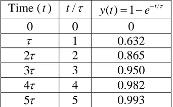
In much of what we do, we will be concerned with the time constants of a system in one way or another. Let’s look at the response of our first order system assuming the system is initially at rest (y(0)=0) and the final value is one ( ). Let’s look at the response of our system as the time t takes on the values of integer number of time constants:

( ) 1

Time (t) t/τ /

( ) 1 t

y t = −e− τ

0 0 0

τ 1 0.632

2τ 2 0.865

3τ 3 0.950

4τ 4 0.982

5τ 5 0.993

Figure 2.6 show this result graphically, The way this information is usually interpreted is that a system is within 5% of its final value in 3 time constants, within 2% of its final value in 4 time constants, and within 1% of its final value in 5 time constants. Hence the use of time constants gives us a quick way to describe one aspect of the behavior of a system. As we will see, as the systems become more complex, the use of time constants indicates which part of the solution is the most important and how the system responds to periodic inputs (sines and cosines).

0 1 2 3 4 5 6 7

0 0.1 0.2 0.3 0.4 0.5 0.6 0.7 0.8 0.9 1

Number of Time Constants

y(

t)

Figure 2.6. Graph of y t( )= −1 e−t/τ for t=0τ up to t=7τ. is within 5% of its final value in 3 time constant, within 2% of its final value in 4 time constants, and within 1% of its final value in 5 time constants.

( )

Example 2.3.1. Consider the circuit in Figure 2.2 (Example 2.1.2). Let’s first assume R_a =R_b =2kΩ

and C=1μF. Then R_th= Ω1k , τ =1ms, and K =0.5. Next we will assume the initial voltage on the capacitor is zero (v t_c( )₀ =v_c(0)=0) and the input is as follows:

0 0

2 0

2 8

8

1 1

( )

16

s

t

v

t t

t t

6 ≤ ≤ =

≤ < ⎧

⎪ ⎪

⎨− < ⎪

⎪ _> ⎩

Here the input is in volts and the time is measured in milliseconds. We now want to determine the output. We will do this by looking at the initial and final values for each time interval, where the time intervals are determined by the times during which the input voltage is constant. The differential equation is

( )

( ) ( )

c

c s

dv t

v t Kv t dt

τ + =

Clearly ( )y t =v t_c( ) and x t( )=v t_s( ). The solution in each interval will be of the form

[

]

( ) (0) ( ) t ( )

y t = y − ∞y e− τ + ∞y

At this point we just need to be able to determine what y(0) and y( )∞ mean for each interval.

First interval (0≤ <t 8 ms) : We have the initial value in this intervaly(0)=vc(0)=0 volts. To determine the final value, we use the static gain and the amplitude of the input for this interval.

1

( ) ( ) 2 2 1

2 c

v ∞ = ∞ =y Ki = i =

Hence for this interval, we have the solution

/ /0.001

( ) ( ) t 1 1 t

c

v t = y t = −e− τ + = −e−

Before we go on to the next interval we need to figure out the value of at the end of this interval, this value will be the initial point during the next interval. At the end of the interval we will have

( )

y t

0.008/0.001 8

1

(0.008) 1 e 0.99966 1.0

y = −e− = − − = ≈

Second interval (8 ms) : The initial value for this interval will be the end point of the previous interval, so . To determine the final value we again use the static gain

16

t

< ≤

1 = (0)

y

1

( ) ( 2) ( 2)

2

K

y ∞ = i − = i − = −1

beginning of the interval from our actual time in our form of the solution, so our time will be measured from the beginning of the interval. Our solution for this interval is then

( 0.008)/ ( 0.008)/0.001

( ) [1 ( 1)] t ( 1) 2 t

y t = − − e− − τ + − = e− − −1 At the end of this interval we will have

(0.016 0.008)/0.001 8

2 1 2 1 0.999

(0.016) e e 33 1.0

y = − − − = − − = − ≈ −

Third interval ( ms): The initial value for this interval will be the end point of the previous interval, so . To determine the final value we have

16

t> (0)= −1

y

1

( ) 1

2

y ∞ =Ki =K =

Again we must scale our solution so time is measured from the beginning of the interval, so we have

( 0.016)/ ( 0.016)/0.001

0.

( ) [ 1 0.5] t 5 1.5e t 0.5

y t = − − e− − τ + = − − − +

Total solution: To get the total solution, we list the solutions during each time interval:

/0.001 ( 0.008)/0.001 ( 0.016)/0.001 1 8 ( ) 2 1 0 0 0 ( ) 8

1.5 0.5 16

t c t t e t t e t t v s y t e t ms − − − − − ⎧ ⎪ _{− ≤} ⎪ = _⎨ − < = + ≤ < ⎪ ⎪− ≥ ⎩ 16 ms m <

To get the current through the capacitor, we use the relationship ( ) c( ) c

dv t i t C

dt

= for each time interval above. Doing this we get

/0.001 ( 0.008)/0.001 ( 0.016)/0.001 0 0 0 8 0.001 8 ( ) ( ) 0.002 16 0.015 16 t c c t t e t dv t t C e t t s dt i t e m − − − − − ⎧

⎪ _{≤ <}

⎪ = _⎨ ≤ < ⎪ ⎪− ≥ ⎩ < = ms m s

Here i t_c( ) is measured in amps.

Figure 2.7 shows the input voltage, the voltage across the capacitor, and the current through the capacitor as a function of time. Note that the voltage across the capacitor is continuous, as it must be. However for this input, which is discontinuous, the current through the capacitor is discontinuous. Let’s also look at the answer to see if we can check our results and if the answer makes sense. When the source voltage is initially turned on, the voltage across the capacitor is zero and all of the voltage generated by the source is equal to the voltage across resistorR_a. If there were any voltage drop across

b

Finally is useful to point out that if the voltage across the capacitor is described by the relationship

/

( ) [ (0) ( )] t ( )

c t vc vc e vc

v = − ∞ − τ + ∞

Then the current through the capacitor is given by

/ ( )

( ) c [ (0) ( )] t

c c

t

t Cdv C v v e

i

dt c

τ

τ

−

− ∞

= − =

What this means is that if the voltage across a capacitor is growing exponentially, then the current through the capacitor is decreasing exponentially. Similarly, if the voltage across a capacitor is

decreasing exponentially, the current through the capacitor will be growing exponentially. This is also behavior our results show. Similar results also hold for inductors.

Example 2.3.2. Consider the circuit in Figure 2.4 (Example 2.1.4). Let’s first assume and

100

th

R=R = Ω

10

L= mH. Then 0.01 0.0001 100 100

L

s R

τ = = = = μ andK=0.01. Next we will assume the initial current through the inductor is i(0)=10mAand the input is as follows:

0 0

2 0 0.1

( )

3 0.1 0.25

4 0.25

s

t t v t

t t

< ⎧

⎪ _{≤ <} ⎪

= ⎨_{− ≤ <} ⎪

⎪ _≥

⎩

Here the input is in volts and the time is measured in milliseconds. We now want to determine the output. We will do this by looking at the initial and final values for each time interval, where the time intervals are determined by the times during which the input voltage is constant.

The differential equation for this system is again

( )

( ) _s( )

di t

i t Kv t dt

τ + =

Clearly y t( )=i t( ) and x t( )=v t_s( ). The solution in each interval will be of the form

[

]

( ) (0) ( ) t ( )

y t = y − ∞y e− τ + ∞y

0 5 10 15 20 25 -2

-1 0 1 2

V s

(t

) (v

ol

ts

)

0 5 10 15 20 25

-1 -0.5 0 0.5 1

V c

(t

) (v

o

lt

s

)

0 5 10 15 20 25

-2 -1 0 1 2

i c

(t

) (m

A

)

Time (ms)

Figure 2.7. Results for Example 2.3.1.

First interval (0≤ <t 0.1ms) : We have the initial value y(0)=i(0)=0.01amps in this interval. To determine the final value, we use the static gain and the amplitude of the input for this interval

1

( ) ( ) 2 2 0.02

100

i ∞ = ∞ =y Ki = i =

Hence for this interval, we have the solution

[

]

( ) (0) ( ) t ( ) [0.01 0.02] t 0.02 0.01 0.02

y t = y − ∞y e− τ + ∞ =y − e− τ + = − e−t +

Before we go on to the next interval we need to figure out the value of at the end of this interval, this value will be the initial point during the next interval. At the end of the interval we will have

( )

y t

0.0001/0.0001 1

(0.0001) 0.01 0.02 0.01 0.02 0.01632

Third interval ( ) : The initial value for this interval will be the end point of the previous interval, so . To determine the final value we again use the static gain

0 0.1≤ <t .25

(0) 0.016

y = ms

.03 32

) 3) 0.01

( K ( ( 3) 0

y ∞ = i − = i − =−

We again need to subtract the time at the beginning of the interval from our actual time in our form of the solution, so our time will be measured from the beginning of the interval. Our solution for this interval is then

( 0.0001)/ ( 0.0001)/0.0001

( 0.03) 0.04632 0.03

( ) [0.01632 ( 0.03)] t e t

y t = − − e− − τ + − = − − −

At the end of this interval we will have

(0.00025 0.0001)/0.0001 1.5

0.04632 0.03 0.04632

(0.00025) e e 0.03 0.01966

y = − − − = − − =−

ms

Fourth interval ( ): The initial value for this interval will be the end point of the previous interval, so . To determine the final value we have

0.25 t≥ 0.01966 = − (0) y

( ) 4 0.04

y ∞ =Ki =

Again we must scale our solution so time is measured from the beginning of the interval, so we have

( 0.0025)/ ( 0.00025)/0.0001

0.

( ) [ 0.01966 0.04] t 04 0.05966 t 0.04

y t = − − e− − τ + = − e− − +

Total solution: To get the total solution, we list the solutions during each time interval:

/0.0001 ( 0.0001)/0.0001

( 0.00025)/0.0001

0.01 0.02 0.1

( )

0.04632 0.03 0.1

0 0 0 0.25 0.05966 0.25 ( ) 0.04 t L t t t e t t e i y t m ms t t e − − − − − ⎧

⎪ _{− + ≤ <}

⎪

= _⎨

− ≤ <

⎪ ⎪− + ≥ ⎩ < = ms s

To get the voltage across the inductor we use the relationship ( ) L( ) L di v L t t t d

= and compute the voltage for each time interval. Doing this we get

/0.0001 ( 0.0001)/0.0001 ( 0.00025)/0.0001 0.1 ( ) ( ) 4.632 0.1 0 0.25 5.966 0 0 0.25 t L L t t t

v e t

t s di t t L e t dt e m − − − − − ⎧

⎪ _{≤ <}

⎪ = _⎨− ≤ ≥ < = ⎪ ⎪⎩ m ms s <

The initial current in the inductor is 10 mA, as we require, and the initial voltage from the source is 2 volts. Applying Kirchhoff’s laws around the loop, we expect the initial voltage drop across the inductor to be given by volts, which is what we have. In steady state the

inductor looks like a short circuit, so there should be no voltage drop across the inductor once the system reaches steady state, which again matches our results. Note that the system only reaches steady state near 0.7 or 0.8 ms. In addition, in steady state the voltage drop across the resistor must match the voltage supplied by the source, or volts, which again matches our results. Let’s look at the results at one other convenient point in time, say

(0) (0) 2 (0.01)(100) 1

s i R

v − = −

( ) ( )

s

v ∞ − ∞i

=

ms 4 (0.04)(100) 0

R= − =

0.2

t = . Using the equations we derived above (and the known input) we have

(0.0002) 3 (0.0002) 12.96

(0.0002) 1.70

s l L

v volts

i m

v volts

A

= − = −

= − Applying Kirchhoff’s laws around the loop we have

(0.0002) (0.0002) (0.0002) 3 ( 0.01296)(100) ( 1.70) 0.0

s s L

v −i R v− = − − − − − ≈

We can obviously check as many points in time as we want in this way. This type of checking does not guarantee our answer is correct, but it does help find obvious errors.

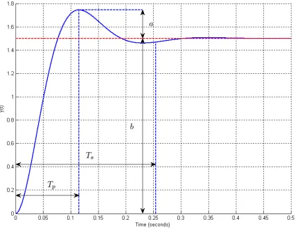
2.3.2 Solution Using Integrating Factors

An alternative method of solution of first order differential equations is by the use of integrating factors. This method of solution is important to understand because as we start to analyze different types of

systems, we need to be able to understand how we would solve for the output when we don’t actually know what the input is. This helps us characterize systems independent of the actual (specific) input. The use of integrating factors for solving first order differential equations is based on the fact that when we differentiate an exponential, we get the same exponential back multiplied by some other term. For example, if x t( )=eφ( )t , then

( ) ( )

( ) t t ( ) ( ) ( )

d d d d

x t e x t

dt dt e dt d

t t

φ φ

t

φ φ

=

= =

In what follows, the method looks fairly lengthy, but with practice most of the steps can be done in your head. Let’s apply this idea to our equation

( )

( ) ( )

dy t

y t Kx t dt

0 0.1 0.2 0.3 0.4 0.5 0.6 0.7 0.8 -4

-2 0 2 4

Vs

(t

) (v

o

lt

s

)

0 0.1 0.2 0.3 0.4 0.5 0.6 0.7 0.8

-20 -10 0 10 20 30 40

iL

(t

) (m

A

)

0 0.1 0.2 0.3 0.4 0.5 0.6 0.7 0.8

-6 -4 -2 0 2 4 6 8

vL

(t

) (v

o

lt

s

)

Time (ms)

Figure 2.8. Results for Example 2.3.2. This method will work better if we rearrange our equation a bit to the form

( ) 1

( ) ( )

dy t K

y t x t dt +τ = τ

Next, we look at differentiating the producty t e( ) φ( )t , where φ( )t will be determined by the differential equation we are trying to solve. This leads to the equation

( ) ( ) ( ) ( ) ( ) ( ) ( )

( ) t t ( ) t t ( ) ( )

d dy t d dy t d

y t e e e e y t

dt dt d

t t

t t

t t d

y

d

φ φ φ φ φ ⎡ φ ⎤

⎡ ⎤ =_⎦ + =

⎣ ⎢_⎣ + ⎥_⎦

( ) ( ) ( ) 1

( ) ( )

dy t d dy t

y t y t

dt dt dt

t

φ

τ

+ = +

Clearly this means that

) 1 ( d d t t φ τ =

Solving this simple equation we get

( )t t

φ τ

=

Now we put this back into our equation above to get

/ / / /

( )

( ) 1 ( ) 1

( ) t t t t ( )

d dy t dy t

y t e e y e e y t

dt dt t dt

τ τ τ τ

τ τ

⎡ ⎤

⎡ ⎤ = =

⎣ ⎦ + ⎢_⎣ + ⎥_⎦

The term on the far right is the same as the left hand side of our differential equation multiplied by t/

e τ , so this must equal the right hand side of our differential equation multiplied by the same thing,

/ / ( ) 1 /

( ) t t ( ) t ( )

d dy t

y t e e y t e x t

dt dt

τ τ τ

τ τ

K

⎡ ⎤ ⎡

⎡ ⎤ = + =

⎣ ⎦ ⎢_⎣ ⎥_⎦ ⎢_⎣ ⎤⎥_⎦

Next we eliminate the middle term to get the exact differential we want

/ /

( ) t t ( )

d K

y t e e x t dt τ τ τ ⎡ ⎤ ⎡ ⎤ = ⎣ ⎦ ⎢_⎣ ⎥_⎦

Finally we integrate from and initial time t₀ with initial value y t( )₀ to final time t with value y t( ),

0 0 / / ( ) ( ) t t t t K

e d e d

d x

d

y λ λ τ λ λ τ λ

λ⎡⎣ ⎤⎦ = τ

∫

∫

The left hand side can be integrated as

0 0 0 / / / / 0 ) ( ) ( ) ( ( t t t t t t K

e d y t e y t e x

d d

d

y λ λ τ λ τ e τ λ τ λ)

λ⎡⎣ ⎤⎦ = − =

∫

∫

t t t

t

K

y t y t e τ e λ τ x λ λd

τ

− − − −

= +

∫

Example 2.3.1. Let’s now look at the same input as before, x t( )=A for with initial condition and

0

t≥

0 0

t = y t( )₀ =y(0). The solution to the differential equation becomes

/ ( )/

0

( ) (0)

t

t t K

y t y e τ e λ τ Adλ

τ

− − −

= +

∫

/ / /

0

( ) (0)

t

t t K

y t y e τ e τ eλ τ Adλ

τ

− −

= +

∫

/ / /

0

( ) (0) t t t

y t y e− τ e− τKA eλ τ λ_λ=

=

⎡ ⎤

= + _{⎣ ⎦}

/ / /

( ) y(0) t e t et 1

y t = e− τ + − τKA⎡_⎣ τ − ⎤_⎦

/ /

) ) 1

( (0 t KA e t

y t = y e− τ + ⎡_⎣ − − τ⎤_⎦ With the substitution y(∞ =) KA, we get

/ /

( ) (0) t ( ) 1 t

y e

y t =y e− τ + ∞ ⎡_⎣ − − τ⎤_⎦ or

[

]

( ) (0) ( ) t ( )

y t = y − ∞y e− τ + ∞y

the same solution as before.

Example 2.3.2. Let’s use integration factors to determine the solution to the differential equation

( )

( ) ( )

dy t

ay t bx t

dt = +

The first thing we need to do is put all of the y terms on the left hand side,

( )

( ) ( )

dy t

ay t bx t dt − = Then we need

( )

d

a d

t t

φ _{= −}

or

( )t at

φ = −

Then we have

( ) at at ( )

d

y t e e x t

dt b

− −

⎡ ⎤ =

⎣ ⎦

0 0 0 0 ( ) ( ) ( ) ( ) t t at

a at a

t t

d

e y d e y t e y t e bx d

d

λ _{λ λ} λ _λ

λ

−

− − −

⎡ ⎤ = − =

⎣ ⎦

∫

∫

or 0 0 ( ) 0 ( ) ( ) ( ) t

a t t at a

t

y t =e − y t +e

∫

Example 2.3.3. Let’s use integration factors to determine the solution to the differential equation

( )

( ) 2 ( )

dy t

ty t x t dt − = Then we need

( ) d t d t t

φ _{= −}

or 2 ( ) 2 t t

φ = − Then we have

2 2

2 2

( ) 2 ( )

t t

d

y t e e x t

dt − − ⎡ ⎤ = ⎢ ⎥ ⎢ ⎥ ⎣ ⎦

Integrating both sides we get

2

2 2 2

0

0 0

2 2 2 2

0

( ) ( ) ( ) 2 ( )

t t t t

t t

d

e y d e y t e y t e x d

d

λ λ

λ λ λ

λ − − − − ⎡ ⎤ = − = ⎢ ⎥ ⎢ ⎥ ⎣ ⎦

∫

∫

or

2

2 2 2

0

0

(

2 2) 2 2

0

( ) ( ) 2 ( )

t t

t t

t

y t e y t e e x d

λ

λ λ

− −

Chapter 2 Problems

2.1) For each of the circuits below:

i) Determine the governing differential equation using Kirchhoff’s Laws and write it in standard form. For part F the output is the voltage across resistor RC.

ii) Determine the time constant and static gain from the differential equation you derive in (i)

iii) For all circuits except F, determine the Thevenin resistance from the ports of the capactor or inductor and verify the time constants.

Answers:

( ) ( )

( ) ( ), ( ) ( ) ( )

( ) ( )

( ) ( ), ( ) ( )

( )

( )

C L

L in a b C b in

b

a a b C b

L

L in C in

a b a b a b a b

a b c b a c C

C

a c

dv t di t

L

i t i t C R R v t R i t

R dt dt

R R R dv t R

di t L

i t i t C v t v t

R R dt R R R R dt R R

R R R R R R dv t

C v t

R R dt

⎛ ⎞

+ = + + =

⎜ ⎟ ⎝ ⎠

⎛ ⎞ ⎛ ⎞ ⎛ ⎞ ⎛ ⎞

+ = + =

⎜ ₊ ⎟ ⎜ ₊ ⎟ ⎜ ₊ ⎟ ⎜ ₊ ⎟

⎝ ⎠ ⎝ ⎠ ⎝ ⎠ ⎝ ⎠

⎛ + + ⎞

+ =

⎜ ₊ ⎟

⎝ ⎠

( )

( ), ( ) ( )

c in

in in C

a c b b

R L dv t R

v t v t v t

R R R dt R

⎛ ⎞ ⎛ ⎞ ⎛ ⎞

+ = −

⎜ ₊ ⎟ ⎜ ⎟ ⎜ ⎟

⎝ ⎠ ⎝ ⎠ ⎝ ⎠

a

2.2) For a simple series RC circuit the response of the system when the input is a unit step is

/ /

( ) 1 t RC 1 t

y t = −e− = −e− τ

The 10-90% rise time, t , as shown below. The rise time is simply the amount of time necessary for the output to rise from 10% to 90% of its final value. Show that for this system the rise time is given by

r

ln(9)

r t =τ

t90

t₁₀

rise time t_r= t₉₀-t₁₀ 90%

10%

t90

t₁₀

rise time t_r= t₉₀-t₁₀ 90%

2.3) For each of the circuits below:

i) Determine the governing differential equation using Kirchhoff’s Laws and write it in standard form. ii) Determine the time constant and static gain from the differential equation you derive in (i)

iii) For all circuits except F, determine the Thevenin resistance from the ports of the capactor or inductor and verify the time constants.

Answers:

( ) ( ) 1

( ) ( ), ( ) ( )

( ) ( ) ( ) 1

( ) ( ) ( ), ( ) ( ) ( ) ( ) ( 1 ) ( ( ) ) ,

a b L L

L in L in

a b a a b a b

C a b L

a b C a in L in

a b a

a c L c

L in

a c b c a b a c b c a b

R t L di t

t t i t V t

R R R dt R R

dv t R R L di t

R R C v t R i t i t v t

dt R R dt R

R R L di t R

i t v t CR

R R R R

R L d

R R dt R R R R R R

i

i V

R dt R

+ = + = + + + + + = + = + _{+ =} + + + + + ( ) ( ) ( ) C b c C a

dv t R

v t v t

dt + = −R in

2.4) Consider a first order sytem described by the differential equation τy t( )+y t( )=K x t( ). a) If the initial value is y(0)=0 and the final value isy(∞ =) 10, what is y(4τ)?

b) If the initial value is y(0)= −2 and the final value isy(∞ =) 8, what is y(4τ)? c) If the initial value is y(0)=1 and the final value isy(∞ = −) 4, what is y(4τ)?

Answers: 9.82, 7.82, -3.90

2.5) An RC circuit has paramters R_th=R_a||R_b, τ =R_thC, K R= _th and is described by the first ordeer equation ( ) ( ) ( ) c c in dv t

t K t

dt v i

τ + =

For this circuit R_a =100Ω, R_b =200Ω, and C=2 mf.The input current is 0 1 0 2 0.2 3 0 0.2 ( ) 0.4 0.4 in t mA

i t t se

t s

mA

mA t sec

≤ ⎧

⎪ _{≤ <}

⎪

⎨ _{≤ <}

≥ = − ⎪ ⎪⎩ c ec

a) Determine an analytical expression for the voltage across the capacitor in each of these regions b) Enter your analytical expression as an anonymous function in Matlab, and simulate the system using Simulink. Show that all three of your answers are identical. Turn in your Matlab (driver file) code and your neatly labeled plots. Be sure to set the initial value of the integrator to zero.

2.6) An RL circuit has paramtersR_th=R_a+R_b +R_c,τ =L R/ _th , K=(R_a +R_b) /R_thand is described by the first ordeer equation

( )

( ) ( )

L

L in

di t

t K t

dt i i

τ + =

For this circuit,Ra =Rb =Rc =10Ω andL=8 mh.The input current is 0 0.02 0 0.03 0.4 0. 0 05 0.4 ( ) 1.0 1.0 in t A A t m t t m

A t ms

≤ ⎧

⎪ _{≤ <}

⎪

⎨ _{≤ <}

a) Determine an analytical expression for the current through the inductor in each of these regions b) Enter your analytical expression as an anonymous function in Matlab, and simulate the system using Simulink. Show that all three of your answers are identical. Turn in your Matlab (driver file) code and your neatly labeled plots.

2.7) For each of the following first order differential equations, use an integrating factor to write as a function of its initial value

( )

y t

0

( )

y t and an integral of the input (plus some other functions)

2

( ) ( ) ( ) ( ) ( ) ( )

1 1

( ) ( ) ( ) ( ) ( ) ( 1)

y t ay t bx t y t aty t bx t

y t y t x t y t y t x t

t t

= + = +

+ = + = −

Answers:

2 2 2 2

0 0

0 0

0

0 0

( ) ( )

( ) ( ) _{2 2}

0 0

1 1 1 1

0

0 0

( ) ) ( ) ( ) ) ( )

( ) ) ( ) ( ) ) ( 1)

( (

( (

a

t t t

a t t a t

t a t

t t t

t t

t t

t t

y t e x d y t e x d

t

y t x d y t e x

y t be y t be

y t y t

t t e d

λ λ

λ

λ λ λ

λ

λ

λ λ λ

⎛ ⎞

⎜ ⎟

⎝ ⎠

− −

− −

⎛ ⎞

− ⎜_⎝ − ⎟_⎠

= + = +

⎛ ⎞ ⎛ ⎞

=_{⎜ ⎟} + _{⎜ ⎟} = + −

⎝ ⎠ ⎝ ⎠

∫

∫

3.0 Second Order Circuits

A second order circuit is a circuit with two effective energy storage elements, either two capacitors, two inductors, or one of each. (In some circuits it may be possible to combine multiple capacitors or

inductors into one equivalent capacitor or inductor.) We begin this section with the derivation of the governing differential equation for various second order circuits. At this point we will focus on circuits that we can put into a standard form. Once we have covered Laplace transforms we will analyze different types of second order circuits. This standard second order form will again allow us to easily determine physical characteristics of the circuit and predict the time response. We then solve the differential equations for the case of a constant input.

3.1 Governing Differential Equations for Second Order Circuits: Standard Form

In this section we derive the governing differential equations that model various RL, RC, and RLC circuits. We then put the governing second order differential equations into a standard form, which allows us to read off descriptive information about the system very easily. The standard form we will use is

2

2 2

( )

( (

(

) )

2 _{n n} ) _n

d dy t

dt d

y t

y t K

t x t

ζω ω ω

+ + =

or

2 2

1 ( ) 2

( ) ( ) ( )

n n

d y t d

y t y t

dt dt Kx t

ζ

ω +ω + =

Here we assume the system input isx t( ) and the system output isy t( ). ωn is the system natural

frequency, which indicates the frequency at which the system will oscillate if there is no dampling. The natural frequencyω_n has units of radians/second. ζ is the damping ratio, which indicates how much damping there is in the system. A damping ratio of zero indicates there is no damping at all. The

damping ratioζ is dimensionless. K is the static gain of the system. For a constant input of amplitudeA (x t( )= Au( )t , where u t( ) is the unit step function), in steady state we havedy t( ) 0

dt = ,

2 2

( ) 0

d y t

dt = , and

. Hence the static gain lets us easily compute the steady state value of the output. To determine the units of the static gain we use

( ) ( )

y t =Kx t =KA

[units of y] = [units of K][units of x] or

[units of K] = [units of y]/[units of x]

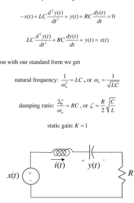
Example 3.2.1. Consider the RLC circuit shown in Figure 3.1. The input, x t( ), is the applied voltage and the output, , is the voltage across the capacitor. If we denote the current flowing in the circuit as , then applying Kirchhoff’s voltage law around the single loop gives us the equation

( )

y t

( )

i t

( ) ( )

) (

( di t y t i t R dt

x t L + +

− + ) =0

We can also relate the voltage across the capacitor with the current flowing through the capacitor

( )

( ) dy t

i t C dt

=

Substituting this equation into our first expression we get

2 2

( ) ( )

0 ( ) d y t y t( ) RCdy t

dt dt

x t LC + +

− + =

or

2 2

( ) ( )

( ) ( )

d y t dy

LC RC t y

dt + dt + t =x t

Comparing this expression with our standard form we get

natural frequency: 1₂

n

LC

ω = , or

1

n

LC

ω =

damping ratio: 2

n

RC

ζ

ω = , or 2

R C

L

ζ =

static gain:K =1

( )

x t

Figure 3.1. Circuit for Example 3.2.1.

Example 3.2.2. Consider the RLC circuit shown in Figure 3.2. The input, x t( ), is the applied current and the output, , is the current through the inductor. If we denote the node voltage at the top of the circuit as , then applying Kirchhoff’s current law give us

( )

y t

*

( )

v t

( )

y t

+ -

-+

( )

i t

* *

( ) ( )

( ) v t y(t) + Cdv t

x t

R dt

= +

We can also relate the voltage across the inductor with the current flowing through the inductor

* ( )

( ) dy t

v t L dt

=

Substituting this equation into our first expression we get

2 2

( ) ( )

( ) L dy t y(t) + LCd y t

x t

R dt dt

= +

or

2 2

( ) ( )

LCd y t L dy t y(t) = x(t)

dt +R dt +

Comparing this expression with our standard form we get

natural frequency: 1₂

n

LC

ω = , or

1

n

LC

ω =

damping ratio:2

n

L R

ζ

ω = , or 1 2

L C R

ζ =

static gain:K =1

( )

x t

R

( )

y t

•

*

v

L

C

Figure 3.2. Circuit used in Example 3.2.2.

Example 3.2.3. Consider the RLC circuit shown in Figure 3.3. The input, x t( ), is the applied current and the output, , is the current through the inductor. If we denote the node voltage at the top of the circuit as , then applyingKirchhoff’s current law give us

( )

y t

*

( )

v t

*

( ) ( ) y(t) + Cdv t

x t

dt

We can then determine the node voltage v t*( ) as

* ( )

( ) ( ) dy t

v t Ry t L dt

= +

Substituting this equation into our first expression we get

2 2

( ) ( ) ( )

( ) ( ) d [ ( ) dy t ] ( ) dy t d

x t y t C Ry t L y t RC LC

dt dt dt dt

= + + = + + y t

or

2 2

( ) ( )

( ) ( )

d y t dy t

LC RC y t x t

dt + dt + =

Comparing this expression with our standard form we get

natural frequency: 1₂

n

LC

ω = , or

1

n

LC

ω =

damping ratio:2

n

RC

ζ

ω = , or 2

R C

L

ζ =

static gain:K =1

R

Figure 3.3. Circuit used in Example 3.2.3.

Example 3.2.4. Consider the RLC circuit shown in Figure 3.4. The input,x t( ), is the applied voltage and the output, y t( ), is the voltage across resistor Rb. Node voltages v and are as shown in the

figure. Applying Kirchhoff’s current law gives at node gives (

a t) v tb( )

( )

a v t

( ) ( ) ( ) ( ) ( ) ( )

0

a a b a a

a

v t x t v t v t v t dv t C

R R R dt

− −

+ + + =

C

•

*

v

L

( )

x t

( )

which we can simplify as

( )

3 ( ) ( ) ( ) a

a b a

dv t v t x t v t RC

dt

− − = −

Summing the currents into the negative terminal of the op amp gives us

( ) ( )

0

a b

b

v t dv t C

R + dt = or

( )

( ) b

a b

dv t v t RC

dt

= −

Substituting this expression into our simplified equation above we get

( ) ( )

3 b ( ) ( ) b

b b a b

dv t d dv t

RC x t v t RC RC

dt dt dt

⎡₋ ⎤_{− − = −} ⎡₋ ⎤ ⎢ ⎥ ⎢ ⎥ ⎣ ⎦ ⎣ ⎦ or 2 2 2 ( ) ( )

3 ( )

b

a b b

b

b

d t dv t

C C RC v t x t

dt dt

v

R + + =− ( )

Finally, we have

)

( ) ( b

b a b R t y v R R t = + or

( ) a b ( )

b b

R R

v t y t

R

+ =

resulting in the differential equation

2 2

2

( ) ( )

3 ( )

a b b

a b

b R

d t dy t

C C RC y t x t

dt dt R

y R

R

+ + = −

+ ( )

Comparing this expression with our standard form we get

natural frequency: 2 2 1

a b n

R C C

ω = , or

1

n

a b R C C

ω =

damping ratio:2 3 _b n

RC

ζ

ω = , or 3 2 b a C C ζ =

static gain: b

Figure 3.4. Circuit used in Example 3.2.4.

3.3 Solving Second Order Differential Equations in Standard Form

In this section we will solve second order differential equations the standard form

2

2 2

2

( )

( (

( ) )

2 _{n n} ) _n

d dy t

dt d

y t

y t K

t x t

ζω ω ω

+ + =

for a constant (step) input. We will solve this equation in two parts. We will first determine the natural response, ( . The natural response is the response due only to initial conditions when no inputs are present. Then we will determine the forced response, . The forced response is the response due to the input only, assuming all initial conditions are zero. The total response is then the sum of the natural and forced responses,

)

n y t

( ) f

y t

( ) _n( ) _f( )

y t =y t +y t .

3.3.1 Natural Response. To determine the natural response we assume there is no input in the system, so we have the equation

2

2 2

( )

) (

(

2 ) 0

n n

n n n

d dy t

dt dt

y t

y t

ζω ω

+ + =

Let’s assume a solution of the form , wherec and are parameters to be determined. Substituting this assumption into the differential equation we get

( ) rt

n

y t =c e r

2 2

2 0

rt rt rt

n n

r ec + ζω rce +ω ce = or

2 2

2 0

[ ]

rt

n n

ce r + ζω r+ω =

+ -

-+

R

R

R

a

R

b

R

b

C

a

C

•

•

v

b

v

( )

x t

-Ifc=0 then we are done, and the natural response will bey t_n( )=0. This solution certainly satisfies the differential equation. However, ifc≠0, and since rt can never be zero, we must have

e

2 2

2 _nr _n 0

r + ζω +ω = Using the quadratic formula, the roots of this equation are

2 2

2 2 2 2

(2 2

) 4

1

2 n n n

n n n n n

r= − ζω ± ζω − ω =−ζω ± ζ ω −ω =−ζω ω ζ± −

We now have four cases to consider depending on