Advanced video debanding

Advanced Video Debanding

Gary Baugh

[email protected]

Anil Kokaram

[email protected]

François Pitié

[email protected]

ABSTRACT

High efficiency video coding has made it possible to stream video over bandwidth constrained communication networks. Depending on bit rate requirements, a video encoder sacrifices some image de-tails which can then introduce visual artefacts. Due to aggressive encoding a contouring staircase artefact called banding can be ob-served in image regions with very low texture. This paper presents a solution for removing banding artefacts using image filtering and dithering techniques. A new banding index (BI) metric is also pre-sented for quantitatively measuring the amount of banding in an im-age. Using this BI metric, we assess how much banding YouTube video encoding introduces in a video test dataset. There is a de-banding filter inffmpegcalledgradfun. We compare the results of our debanding technique with those ofgradfunon the YouTube test dataset.

Categories and Subject Descriptors

I.4.3 [Image Processing and Computer Vision]: Enhancement

General Terms

debanding,online video,encoding artefacts

Keywords

debanding,ffmpeg,enhancement,filtering,segmentation,dithering

1.

INTRODUCTION

Streaming video over a communication network requires that the data rate does not exceed the available bandwidth. On the internet, the bandwidth available to the typical user is usually not sufficient for delivering high bit rate video. Hence, the source material is en-coded to produce a lower bit rate version for streaming. YouTube for example, uses H.264 and VP9 codecs for video content encod-ing. There may be offline constraints such as disk storage capacity which determine that all source content must be encoded at a cer-tain bit rate to minimise disk usage. Video encoding in these sce-narios is lossy, so there is a reduction in video quality with respect

Permission to make digital or hard copies of all or part of this work for personal or classroom use is granted without fee provided that copies are not made or distributed for profit or commercial advantage and that copies bear this notice and the full citation on the first page. Copyrights for components of this work owned by others than ACM must be honored. Abstracting with credit is permitted. To copy otherwise, or republish, to post on servers or to redistribute to lists, requires prior specific permission and/or a fee. Request permissions from [email protected].

CVMP’1413-14 November 2014, London, United Kingdom Copyright 2014 ACM 978-1-4503-3185-2/14/11 ...$15.00. http://dx.doi.org/10.1145/2668904.2668912.

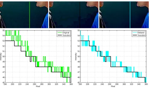
to the source. The bottom left image in Fig. 1 shows a frame from a sequence (SP111) that was uploaded to YouTube. The bottom center image is the YouTube encoded version of this source frame. Also, these pictures are shown in the corresponding row above with some contrast enhancement. There are obvious degradations in the YouTube frame. Some of the textured details on the gray wall is lost (see top row). This is a typical sacrifice in quality the encoder makes in order to meet the bit rate constraint. On image surfaces with relatively slow changing gradients such as this wall, the en-coder will create a staircase artefact as shown in Fig. 1 top center. Here, the contours formed by pixels with the same intensity level is what is referred to as banding. Details of the staircase effect are shown in Fig. 2 for a 1D slice of the image.

The aim of this work is to remove this banding artefact that arises from video encoding.

Importance of Debanding.Although encoded video may con-tain banding artefacts, they may not be observed by the content viewer. The size and quality of the viewing display are major factors here. Also the distance to the display and the amount of ambient light in the viewing environment are significant factors as well. However, with the ever improving quality of displays (such as Retina displays by Apple) in portable devices, the chances of observing banding artefacts are increasing. The viewer is usually positioned close to the display which also increases the odds.

For online premium video on demand services such as Netflix, iTunes and Google Play, video quality and bandwidth preservation are important issues. The consumer of these services indirectly correlates video quality with quality of service. Obvious artefacts such as banding would point toward poor video quality. Therefore, giving the viewer the illusion of a better quality video through de-banding can maintain brand reputation. The dede-banding process can take place after decoding on the client side, so there is no extra demand for bandwidth.

Figure 1: Frame 100 from the Artbeats SP111 sequence.Bottom row: The original (left), YouTube (middle), and debanded (right) versions of this frame.Top row:Contrast enhancement of the corresponding frames in the bottom row.

180 200 220 240 260 280 300 320 340 360 45

46 47 48 49 50 51 52 53 54 55

Pixel

Intensity

Original Youtube

180 200 220 240 260 280 300 320 340 360

45 46 47 48 49 50 51 52 53 54 55

Pixel

Intensity

Deband Youtube

level of quantization they can deal with, or by the picture qual-ity they can achieve. For instance, the debanding plugin in the

ffmpegsoftware is only suitable for very mild cases of banding as its performance degrades very quickly with the quantization lev-els. The restoration can blur the original video, which then looses its details and crispness. Other solutions such as Jin et al [6] are fast but incomplete as they leave a significant amount of blocking artefacts. Also this work makes assumptions specific to the de-coder (H.264/AVC in this case). It is however common practice to transcode a video with several different codecs along a pipeline. Some of these transcoding steps may be unknown, especially for public user generated content. Therefore a generic debanding solu-tion is required that does not need informasolu-tion about prior encoding steps.

Contributions.The first contribution of this paper is to propose a post-processing debanding method which is 1) able to scale with the quantization level, ie. which is able to work with both heavily compressed and high quality videos, 2) conservative, i.e. produce very little artefact of its own, such as over smoothing the entire pic-ture and 3) temporally consistent to avoid any flickering artefacts.

The second contribution of this paper is a technique to detect and report whether a sequence contains banding artefacts. For the debanding stage to exist in a video processing pipeline, there must be metrics to indicate when debanding is required. If no banding is detected the sequence passes through unaltered. We present a new banding index (BI) metric in section 2 for quantifying the amount of banding artefacts in an image.

Organisation of the paper. Our banding metric is presented in section 2 and the debanding algorithm in section 3. The perfor-mance of the debanding algorithm is quantitatively evaluated and compared againstgradfunin section 4.

2.

BANDING INDEX

Human identification of banding artefacts is a difficult task. Not only is this a subjective process, but there is a strong dependence on display quality and size, and environmental conditions. Prior to this work there has not been any published objective metrics for assessing banding in natural images. The metric presented here is called banding index (BI). The BI metric has a strong correlation to the visual perception of banding. Similar to SSIM[8] used for assessing image quality, the BI metric is between 0 and 1. For an image with no banding artefactsBI=1.

Banding is usually observed in image regions with very smooth or uniform regions. The gray wall in Fig. 2 and the blue sky in Fig. 4 are typical examples. The third row of Fig. 4 shows a seg-mentation of the colours for the frames in the row above. Here a segment/block is a group of connected pixels with the same RGB colour. A random colour indicates each block. It may be observed that the YouTube segmentation (center) contains relatively large blocks in the sky, compared to the original (left) and debanded (right) segmentations. The block size is defined as the number of pixels in each segment/block. The distribution of these block sizes in shown the bottom row of fig 4.

The distribution of the block sizes (Fig. 4) provides an indication of the presence of banding artefacts. Therefore the banding index (BI) is based on this observation. For a pixelxwe defineb(x)as the pixel banding index, which is given as,

b(x) = 1

1+e−λ/Ω(x) (1) WhereΩ(x)is the size of the block that contains pixelxandλis a

constant. Fig. 3 shows a plot of the pixel banding indexb(x)versus the block sizeΩ(x), where the constantλ =61.1. The constant

0 20 40 60 80 100

0.65 0.7 0.75 0.8 0.85 0.9 0.95 1

Block Size, Ω(x)

Pixel Banding Index, b(x

)

Figure 3: Plot of pixel banding indexb(x)versus block size

Ω(x)for the constantλ =61.1.

λ=61.1 is chosen so the functionb(x)starts rolling off towards 0

whenΩ(x) =10 (10 pixels). From the distribution of block sizes

for images with out banding, it is observed that the majority of the block are smaller than 10 pixels.

The banding index (BI) is defined using the pixel indexb(x)from Eq. 1 for an image withNpixels,

BI= 1

N

∑

b(x) (2)

Based on experimental results, generallyBI<0.9 indicates the presence of banding. The first two rows in Fig. 4 show an example sequence (SP136) and the corresponding BI metrics. The left col-umn shows the original frame withBI=0.999, which means there is no banding. The YouTube version of this frame is in the center and hasBI=0.834, indicating the presence of banding. Here the banding can be seen in the sky. Finally, the debanded version is on the right withBI=0.996. This suggests that a significant amount of the banding artefacts in the sky have been removed.

3.

BANDING REMOVAL

Similarly to previous works, our debanding algorithm starts by finding the regions in the frame which suffers from banding arte-facts, then applies some filtering correction to these regions to smooth out the bands, and finishes off with a dithering step.

3.1

Detection Mask

The first step is thus to isolate the problematic areas. A bi-nary mask for identifying banding regions can be derived from the colour image segmentation obtained in the banding index evalua-tion. We mark as non-banding region the blocks that have less than 10 pixels in size. Isolated small segments that are not adjacent to any other small segment are discarded and marked as banding.

BI=0.999

BI=0.834

BI=0.996

−10 0 1 2 3 4

1 2 3 4 5 6

log(Block Size)

log(Frequency)

−10 0 1 2 3 4

1 2 3 4 5

log(Block Size)

log(Frequency)

−10 0 1 2 3 4

1 2 3 4 5

log(Block Size)

log(Frequency)

The example frame on the right of Fig. 5 would be a case where minimal correction is required (see detection mask in bottom row).

3.2

Smoothing

With the regions of banding identified in the detection mask, the next step is to smooth out the banded regions to restore the original intensity gradients.

Consider a particular segment/block of the colour segmented im-age. All the pixelsxin the block have similar colourI. The first observation is that for each of these pixels, the original, unbanded, colourˆI(x)cannot differ from the observed pixel colourIby more than some distance, i.e.kˆI(x)−Ik<T. The thresholdT is defined by the quantization process.

The second observation is that within a segment, the colour is probably bounded by the colours of the neighbouring segments. For instance, if we consider the case of a single neighbouring seg-ment (A) with colourIa, then it is likely that the original unbanded colours lie in between both coloursIandIa:

ˆI(x) =w(x)I+ (1−w(x))Ia ,0≤w(x)≤1 (3)

This is simply generalized for more than one neighbour as follows,

ˆI(x) =∑kwk(x)Ik

∑kwk(x)

,wk(x)>0 (4)

The problem is now to suitably define the weightswk.

To achieve some smoothness across segments, we propose to de-sign the weights as a function of the distance from the positionxto a particular neighbouring segmentk. In other words, we wantwk

to get bigger asxgets closer to segmentk. This distance is denoted asd(x,k)and is simply the distance of the nearest pixel in segment

kto pixelx(see Fig. 6).

We also assume that segments with large sizeΩk should have

more influence than smaller segments. Combining all these ideas together, we propose the following definition for the weights,

wk(x) =

  

2

1− 1

1+d(x,k)−Ωk/Ω0

ifkI−Ikk<T

0 otherwise

(5)

whereΩ0denotes the size of segment containingx. These weights

are thus designed so thatwk→0 asd(x,k)→∞. Also the term Ωk/Ω0ensures that small blocks of pixels maintain most of their

original colour when they are surrounded by very large blocks. This is a way of preserving the small details from the source image.

For computational considerations, we argue that we do not need to include all neighbouring segments in the computations. It has been observed in real images that each segment usually has a max-imum of two neighbouring segments. We have thus limited our-selves to the nearest two segments for whichkI−Ikk<T.

In our experiments, we found thatT=20 for colours in the 0:255 range was a good default.

3.3

Dithering

The final correction step involves adding local texture to the smoothed image regions using a dithering technique. From the smoothing step, the imageˆIobtained has floating point precision. However, the final debanded images are often only 8-bits per chan-nel. Going from floating point to 8-bit precision can reintroduce banding artefacts. Therefore, dithering[1, 2, 5] is a commonly used technique for compensating for this lost in precision. The final colour for pixelxis given asIf(x)below,

If(x) =ˆI(x) +η(x)

  1 1 1   (6)

D

A

B

C

x

Figure 6: Distances d(x, .) for pixel x to neighbouring seg-ments/blocks A, B, C and D.

ϒ= 1

16

   

0 8 2 10 12 4 14 6

3 11 1 9 15 7 13 5

   

Whereϒis the dithering kernel, andη(x) =ϒ(xmod4,ymod4), for the pixel coordinatesx= (x,y). Each colour channel inIf(x)is

rounded off to the nearest 8-bit value.

Only the pixels in the banding regions are smoothed and dithered.

4.

EVALUATION

The aim of this work is to improve on the quality of the result obtained from thegradfun debanding filter inffmpeg. To dis-tinguish between our debanding result and that ofgradfunwe will refer to our technique asdeband. Thegradfunfilter is an imple-mentation of a box blur spatial filtering technique. Gradfunalso does dithering of the final image to compensate for the 8-bits per channel precision offfmpeg.

4.1

Visual Comparison

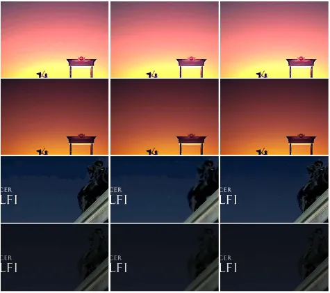
Some of the differences in performance betweengradfunand de-bandare visually obvious. Fig. 7 shows the debanding results for both techniques on images from theMemphisandHouse of Cards

Figure 7:Left column:Frames from theMemphis(1280×720) andHouse of Cards(1920×1080) sequences.Center column:The result ofgradfuntechnique.Right column:The result of ourdebandtechnique. Contrast enhanced images are in the odd rows.

TheHouse of Cardssequence in the bottom row of Fig. 7 con-tains more challenging banding artefacts. The banding contours are relatively larger here (left column) compared to theMemphis

sequence.Gradfunfails to remove the bands in theHouse of Cards

sequence. See the center image in third row for the contrast en-hancedgradfunresult. It may be observed that the edge details are very blurred compared to ourdebandresult on the right. Our de-bandresult in the right column shows that all the banding artefacts are completely removed and we again preserve all the edge details. Note that the stars in the blue sky are quite sharp.

4.2

YouTube Experiment

To perform an objective quantitative analysis between the re-sults ofdebandandgradfun, we uploaded 36 high quality video sequences to YouTube. We obtained theYouTubeencoded versions of these videos, which are then debanded usinggradfunand our

debandtechnique. The high quality version of each sequence is referred to as theoriginalin subsequent discussions.

The 36 test sequences (PAL resolution, 720×576) are from the

Artbeatsvideo collection, which is available online at,

artbeats.com/collections/362-Sports-1

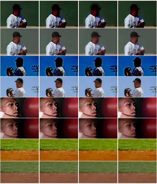
There is a total of 18827 frames from all 36 sequences, which are calledSP101, SP102, ..., SP136. Fig. 8 shows frames from theSP101,SP101,SP112,SP122andSP110sequences. The first and second columns contain theoriginalandYouTubeimages re-spectively. It may be observed that there is visible banding in the

YouTubeimages for the top three sequences. Again contrast en-hancements are provided in rows one, three, five and seven for viewing the banding artefacts.

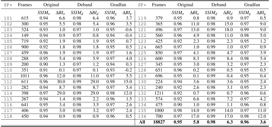
Table 1: Comparison oforiginal,debandandgradfunsequences with respect to the correspondingYouTubesequences.

SP* Frames Original Deband Gradfun SP* Frames Original Deband Gradfun

SSIMo ∆BIo SSIMd ∆BId SSIMg ∆BIg SSIMo ∆BIo SSIMd ∆BId SSIMg ∆BIg

101 615 0.94 6.6 0.98 6.4 0.96 3.7 119 379 0.95 0.8 0.98 0.9 0.97 0.5

102 300 0.95 5.5 0.98 5.4 0.96 3.5 120 365 0.96 11.0 0.98 15.0 0.97 9.0

103 324 0.93 1.0 0.97 1.0 0.95 -0.6 121 496 0.97 13.0 0.99 18.0 0.99 9.0

104 149 0.94 0.9 0.97 0.8 0.94 -0.4 122 560 0.96 4.9 0.98 11.0 0.98 5.0

105 719 0.92 1.9 0.98 1.9 0.95 0.7 123 425 0.92 2.3 0.98 2.3 0.95 1.2

106 900 0.92 1.8 0.98 1.8 0.95 0.5 124 665 0.97 1.0 0.99 1.0 0.97 0.9

107 459 0.96 1.9 0.99 1.9 0.97 1.6 125 850 0.97 4.1 0.98 4.7 0.97 3.9

108 288 0.95 5.4 0.98 5.9 0.97 4.0 126 600 0.98 8.3 0.99 8.4 0.98 5.4

109 200 0.90 1.3 0.97 1.2 0.94 0.3 127 345 0.95 3.0 0.98 3.2 0.97 2.3

110 351 0.91 0.1 0.97 0.1 0.93 -0.2 128 651 0.96 0.2 0.99 0.5 0.95 0.5

111 1011 0.96 12.0 0.98 11.0 0.97 5.5 129 696 0.95 0.1 0.99 0.4 0.95 0.4

112 611 0.96 30.0 0.99 29.0 0.98 15.0 130 224 0.94 3.6 0.98 3.6 0.95 2.4

113 282 0.94 8.7 0.98 8.7 0.97 5.4 131 240 0.92 2.6 0.98 3.1 0.95 2.3

114 398 0.97 29.0 0.99 29.0 0.98 12.0 132 1211 0.92 0.7 0.99 0.7 0.96 0.6

115 267 0.94 1.4 0.98 2.2 0.96 1.5 133 574 0.92 6.6 0.98 7.2 0.97 4.2

116 641 0.95 3.4 0.98 3.5 0.97 2.6 134 475 0.90 1.0 0.99 1.1 0.96 0.8

117 406 0.95 3.0 0.98 3.2 0.97 2.4 135 1000 0.98 14.0 0.99 14.0 0.97 11.0

118 450 0.94 0.9 0.98 0.9 0.96 0.5 136 700 0.97 17.0 0.99 17.0 0.98 12.0

All 18827 0.95 5.8 0.98 6.3 0.96 3.6

in that sequence. The percentage change in the banding index∆BI

is defined as,

∆BIv=

BIv−BIy

BIy

×100% (7)

WhereBIyis the banding index of the aYouTubesequence, and

v∈ {o,d,g}for the correspondingoriginal,debandandgradfun

versions of this sequence.

We also measure the change in picture quality using the popu-lar SSIM metric[8]. The quantitiesSSIMo,SSIMd andSSIMgare

defined as the similarity of theoriginal, debandand gradfun se-quences with respect to theYouTubeversion.

4.2.1

Results

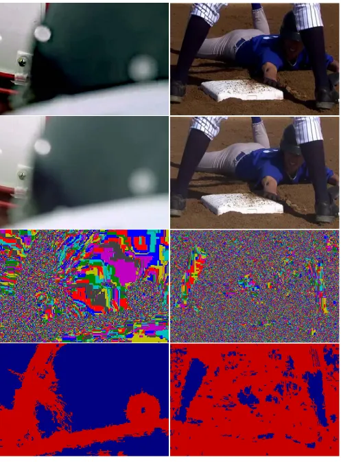
Table 1 summaries the results for the 36 test sequences. Se-quenceSP112had the most banding artefacts due to YouTube en-coding. Frames from this sequence are shown in rows three and four (from top) of Fig. 8. The enhanced YouTubeimage in the third row, second column shows that there is significant banding in the blue sky behind the baseball pitcher. The majority of the frame is occupied by the background sky, which is a prime candi-date for having banding artefacts. Hence a banding index change

∆BIo=30% is a justified result. Ourdebandtechnique removed

the majority of the banding for this sequence. This is supported by the corresponding visual result in the fourth column of Fig. 8, as well as a∆BId=29% value. The corresponding banding change

forgradfun is∆BIg=25%. The visual result forgradfun(third

column) has the edge halo artefact discussed earlier for the Mem-phissequence. This artefact also exist in the results for theSP101

sequence in the top two rows.

SequenceSP110with a banding change∆BIo=0.1% in table 1

has the least banding artefact due to YouTube encoding. The bot-tom two rows of Fig. 8 shows images from this sequence. The contrast enhanced images are in the second row from the bottom. Theoriginalframe in the first column shows that this sequence is highly textured. The majority of the frame is occupied by grass and soil. Hence, there is enough local variations in the intensity here to

prevent banding artefacts. Thegradfunversion of this sequence in the third column is very blurred. This is not the case for ourdeband

result in the fourth column. The blurring ofSP110bygradfun in-troduces some slight banding artefacts, which is supported by the banding change∆BIg=−0.2% value. We again see blurred results

bygradfunfor theSP122sequence in rows five and six in Fig. 8. According to the last row of table 1, ourdebandtechnique made an overall improvement in the banding index of 6.3% compared to 3.6% bygradfun. Alsodebandmade less changes to theYouTube

images as suggested by a meanSSIMd=0.98 compared togradfun

with a valueSSIMg=0.96. This means that we preserve more of

the source image. The amount of banding introduced by YouTube encoding was overall∆BIo=5.8%. This was roughly the amount

removed bydeband∆BId=6.3%. Some of theoriginalsequences

contained some banding artefacts which accounts for the difference in the amount introduced versus removed. Eventhough, the origi-nalvideos were encoded at a high bit rate, the encoding process unavoidablely introduced some banding artefact.

5.

CONCLUSION

We presented a technique for removing banding artefacts from video sequences. This quality of the result produced by our de-bandtechnique is a significant improvement over the current de-banding solution (gradfun) inffmpeg. Unlikegradfun, ourdeband

technique does not create any visible visual artefacts in the final restoration. We also introduced a new banding index (BI) metric for assessing the amount of banding in an image. Using this BI metric, we were able to quantify the amount of banding the Youtube encod-ing process introduced into a test video dataset. The performance of our proposeddebandtechnique outperformedgradfunin terms of the amount of banding it was able to remove from the YouTube video dataset.

floating point precision. For future work we can improve the per-formance of our filter be doing a multithreaded implementation and reducing the number of floating point operations.

6.

REFERENCES

[1] L. Akarun, Y. Yardunci, and A. Cetin. Adaptive methods for dithering color images.Image Processing, IEEE Transactions on, 6(7):950–955, Jul 1997.

[2] B. Bayer. An optimum method for two-level rendition of continuous-tone pictures.Image Processing, IEEE Transactions on, 6(7):11–15, Jun 1973.

[3] S. Bhagavathy, J. Llach, and J. Zhai. Multiscale probabilistic dithering for suppressing contour artifacts in digital images.

Image Processing, IEEE Transactions on, 18(9):1936–1945, Sept 2009.

[4] S. Choy, Y. Chan, and W. Siu. Reduction of block-transform image-coding artifacts by using local statistics of transform coefficients. 4(1):5–7, January 1997.

[5] R. S. Gentile, E. Walowit, and J. P. Allebach. Quantization and multilevel halftoning of color images for near-original image quality.J. Opt. Soc. Am. A, 7(6):1019–1026, Jun 1990. [6] X. Jin, S. Goto, and K. N. Ngan. Composite model-based dc

dithering for suppressing contour artifacts in decompressed video.Image Processing, IEEE Transactions on,

20(8):2110–2121, Aug 2011.

[7] Y. Lee and H. Park. Loop-filtering and post-filtering for low bit-rates moving picture coding. InImage Processing, 1999. ICIP 99. Proceedings. 1999 International Conference on, volume 1, pages 94–98 vol.1, 1999.

[8] Z. Wang, A. Bovik, H. Sheikh, and E. Simoncelli. Image quality assessment: from error visibility to structural similarity.Image Processing, IEEE Transactions on, 13(4):600–612, April 2004.