Resource Virtualization for Customized
Delay-Bounded QoS Provisioning in Uplink
VMIMO-SC-FDMA Systems
Xiaofeng Lu, Qiang Ni, Danping Zhao, Wenchi Cheng, and Hailin Zhang
Abstract—Wireless Network Virtualization (WNV), which de-couples the physical supply process and the service provisioning process, can abstract, isolate and share the physical infras-tructure network equipment. This paper studies the resource virtualization in virtual multiple-input multiple-output single-carrier frequency-division-multiple-access (VMIMO-SC-FDMA) uplink systems, where resources are abstracted to hide the complex details of the fading channel and the link rates are virtualized using the statistical method. Furthermore, the virtual link rates are scheduled and instantiated to different slices with customized delay-bounded quality of service (QoS) provisioning. In this scheme, physical mobile network operator (PMNO) is in charge of the network resource at the physical layer while virtual mobile network operators (VMNOs) are responsible for the traffic admission and the slice management at the MAC layer. Furthermore, we build up the resource virtualization problem as a cross-layer Stackelberg game, which has the interactive dual processes based on the QoS exponent: top-to-down sub-game of leaders at the MAC layer and down-to-top sub-game of follower at the physical layer. Using the newly designed functions for PMNO and VMNOs, we develop an effective dynamic algorithm with iterative dual update to meet the optimization targets of PMNO and VMNOs. Simulation results verify the superiority and stability of delay-bounded QoS guaranteed wireless resource virtualization algorithm developed in this paper in terms of convergence, access rate, and delay-outage probability.
Index Terms—Wireless resource virtualization, Stackelberg game, effective bandwidth, effective capacity, resource allocation, admission control.
I. INTRODUCTION
W
NV is regarded as a key networking paradigm for di-verse network services over a shared wireless network infrastructure [1]. A representative wireless virtual network is composed of PMNOs and VMNOs. PMNO is in charge of network infrastructures such as frequency spectrum, band-width resource and so on, while the underlying resources owned by a PMNO are abstracted and isolated into multiple virtual resource (VR) slices. VMNO, which has no physical substrate, rents the VR slices and corresponding functionalities supplied by PMNO, and then operates the allocated VR slicesThis work was supported by the National Natural Science Foundation of China (61371127 & 61572389 & 61671347 & U1705263), the Key Research and Development Plan of Shaanxi Province (2018ZDCXL-GY-04-06), the EU FP7 CROWN Project under Grant Number PIRSES-GA-2013-610524 and the Royal Society project IEC170324.
Xiaofeng Lu(e-mail: [email protected]), Danping Zhao, Wenchi Cheng and Hailin Zhang are with State Key Laboratory of Integrated Services Networks, Xidian University, China. e-mail:([email protected]).
Qiang Ni is with School of Computing and Communications, Lancaster University, LA1 4WA, U.K. (e-mail: [email protected]).
to provide more flexible and customized QoS to their end users independently.
For next generation wireless systems, VMIMO techniques are expected to increase capacity by spreading the spatial resources among multiple users, especially for uplink systems. Since a base station (BS) usually knows downlink data infor-mation, downlink resource is easy to be allocated. Then in this paper, VMIMO-SC-FDMA uplink systems are studied for the WNV, where a BS serves multiple users within its coverage. From a PMNO’s perspective, its network node such as a BS is partitioned into slices, and each of them represents a virtual mobile network (VMN).
The following aspects need to be considered in the design of WNV:
• Slice isolation: As multiple slices with different require-ments coexist in the system, the first problem is the isolation of these slices. In other words, any change in one virtual slice should not introduce any interference to other slices. In addition, there are many levels of isolation, such as the lowest level on hardware, flow level on time-slot, application level on traffic, etc. In this paper, slice isolation is implemented at the MAC layer with virtual link rate, and the customized delay-bounded service of each slice is independent.
• QoS and delay: The purpose of VMNs is to provide flexible and customized services to end users, and there may be many services with different traffic characteristics in VMNs.
• Slice resource requirement and allocation efficiency: An-other issue is how to meet the different requirements of all slices simultaneously and allocate the resources efficiently.
The technical aim of the paper is to propose an efficient resource reservation algorithm for WNV with delay-bounded QoS guarantee. There are three goals to be achieved in this paper: virtual network isolation, efficient resource allocation and per-flow delay-bounded QoS guarantee. Compared with the existing literatures on WNV, this paper has the following major contributions:
under the condition of given initial channel state. Based on the finite-state Markov channel (FSMC) model and QoS exponent method, we abstract the resources reserved on the link by using average rate to hide the random characteristics of the fading channel so that effective bandwidth (EB) can be used for virtual rate splitting and sharing. Correspondingly, to instantiate the virtual link service rate, effective capacity (EC) is used to give the actual service capability with specific QoS exponent. • To formulate the resource virtualization problem as a
multi-leader single-follower Stackelberg game, where the VMNOs are considered as the leaders while the PMNO as the follower. The follower sub-game performs resource reservation to meet the data service rate requirements from VMNs, and the leader sub-game maximizes the individual utilities of different VMNOs with the spe-cial delay-bounded QoS constraints. During the resource reservation process, the spatial domain of VMIMO and time-frequency domain of adjacent time-frequency re-source blocks (RBs) are virtualized and instantiated. • To develop an iterative cross-layer dual update algorithm
to the solution of the virtualization problem, and to address the rate gap between virtualization and instan-tiation, we design the convex utility functions of PMNO and VMNOs, and we propose an iterative algorithm to dynamically adjust the traffic admission and conjectural service rate until they converge to the Stackelberg Equi-librium.
The rest of this paper is organized as follows. We give a review of the related research work in Section II. Section III describes the system model in terms of VMIMO-SC-FDMA systems and further clarifies the problem solved in this paper. Section IV formulates the above delay-constrained resource virtualization as a Stackelberg game. Section V presents the algorithmic solutions to the formulated problems and the exis-tence of Nash Equilibrium. Section VI presents the simulation results. The conclusions are stated in Section VII.
Here are some notations to be used in this paper : • P (·): probability operation.
• Im,1m×n:m×midentity matrix andm×nmatrix with
all 1’s, respectively. • ⊗: Kronecker product.
• (•)T,(•)H: Transposition, Hermitian, respectively. • [•]u,u: elements at theu-th row and theu-th column of
a matrix.
• E [•]: expectation operation.
Throughout this paper, all matrices and sets are denoted by capital letters in boldface, and vectors are denoted by lowercase letters in boldface.
II. RELATED WORK
A. Wireless Resource Virtualization
With the gradual ossification of the Internet, network vir-tualization has emerged as an important potential solution, and enables deploying customized services on a shared in-frastructure. The authors in [2], [3] provide brief surveys on some existing works about wireless virtualization, and
also mention the challenges and future directions. Further, in [4], J. van de Belt et al. first revisit several key concepts about wireless network virtualization and clarify the difference between abstraction and representation. Then, they develop a theory of virtualization to discuss virtualization in a coher-ent and structured manner. In existing architectures, wireless network infrastructures, especially in radio access network (RAN) [5-12], are sliced to create wireless virtual resources, which can offer customized services to VMNs by different schedulers in a secure and isolated manner. M. Yanget al. only propose OpenRAN, an architecture for software-defined RAN via virtualization [5]. L. Zhao et al. propose an air interface virtualization scheme in LTE system, and further study the time-frequency PRB allocation problem for different traffic models [6], [7]. In [8], R. Kokkuet al. propose and implement a network virtualization substrate for effective virtualization of wireless resources in WiMAX cellular networks. The design provides flow-level virtualization on time-slot to foster a broad set of deployment scenarios and meets the requirements of isolation, customization and resource utilization. Though the above research works have been carried out on wireless resource virtualization, channel status is neglected in network virtualization widely. Further, the authors in [9], [10] study the resource measurement and allocation problems on a flat fading channel. Specifically, in [9], X. Zhanget al. propose an information-centric wireless network virtualization technique for the time sensitive multimedia data transmission problem, where the diverse delay-bounded QoS is measured by the EC theory. In [10], F. Fu et al. present a new wireless network virtualization framework to support multiple heterogeneous self-interested services over the same physical network. In detail, they model the dynamic interactions among service providers (SPs) and the network operator (NO) as a stochastic game, where the NO focuses on the efficient dynamic resource allocation by abstracting the underlying channel conditions via a time-varying feasible rate region, while SPs only focus on their own service objectives and constraints. The algo-rithms proposed in [9], [10] are for flat fading channels, but cannot be directly applied to the actual broadband wireless communication system, where channels are with frequency-selective fading channels. Thus, to address this issue, we have done some research works on resource virtualization in orthogonal frequency division multiplexing access (OFDMA) systems under a frequency-selective wireless channel [11], [12], where the virtual resource slices are implemented on subcarrier at the physical layer. However, the delay-bounded QoS provisioning and the virtualization of multi-dimensional resources, such as spatial and time-frequency resources, are not considered. In this paper, we provide a multi-dimensional resource virtualization mechanism. To describe simply, we focus on the resource virtualization in uplink VMIMO-SC-FDMA systems, which can be easily extended to other systems such as MIMO-OFDMA systems.
B. EC and EB
of low delays have emerged, such as popular multimedia applications. To characterize the effect of delay on the system, two important concepts, EB [13] and EC [16], have been proposed for matching the source traffic arrival process and the network service process respectively. In [13]-[15], EB has been developed to model the statistical behaviour of traffic. In particular, the theory shows that the queuing constraints are imposed on buffer violation probabilities and specified by the QoS exponent, which indicates the exponential decay rate of the QoS violation probability. Inspired by EB theory,
Wu et al. define the concept of EC, which provides the
maximum constant arrival rate that can be supported by a given channel service process while satisfying a statistical QoS requirement specified by the QoS exponent [16]. The analysis and application of EC in various settings have attracted much interest recently [17]-[19]. Since EB and EC mentioned above facilitate capturing the delay-bounded constraint of wireless link without going into complex queuing analysis, we use these dual concepts to characterize the delay-bounded constraints in our cross-layer resource virtualization scheme.
C. Wireless Channel Model and VMIMO-SC-FDMA
The FSMC model has been widely used to model the wireless fading channel mathematically, which is analytically tractable and can provide closed-form results. Specifically, a useful FSMC model is designed to represent the Rayleigh fading channel according to the received SNR [20]. In [21], M. Hassan et al. propose a new partitioning approach that results in a FSMC model with tractable queuing performance. The authors in [22] introduce the Gauss-Markov model to describe the MIMO channel matrix and derive the bounds of the ergodic capacity in closed-form. Similarly, S. H. Ting et al. [23] propose a Markov-kronecker model for analysis of time varying channel in MIMO systems.
VMIMO, also called multiuser MIMO, refers to a com-munication system where a BS with multiple antennas serves two or more single antenna users on the same frequency band and time slot. Compared with the conventional MIMO system, VMIMO can obtain additional multiuser diversity gain by grouping users using well-designed strategies [24]-[26].
In order to obtain both multiuser diversity gain and fre-quency selective gain, VMIMO is usually applied to uplink SC-FDMA systems [24]-[26]. In [24] and [25], joint resource allocation algorithms are proposed for uplink VMIMO-SC-FDMA systems with fixed 2-user pairing. In [26], dynamic user grouping and joint resource allocation algorithm is pro-posed for multi-cell uplink VMIMO-SC-FDMA systems.
D. Stackelberg Game
The Stackelberg model, also known as “leader-follower model”, is a first-mover advantage model in which the leader first takes advantage of the competition. To date, Stackelberg game has been considered as a powerful tool to analyze in-teractive decision-making processes in the resource allocation problems, and has been extensively studied and adopted in various fields. Specifically, in [27], K. Zhu et al. formulate the power control hierarchical competition between the macro
BSs and small cell BSs as a distribution-free multi-leader multi-follower robust Stackelberg game, where the MBSs are the players of the sub-game and the SBSs are the players of the follower sub-game. In [28], [29], H. zhang et al. model the resource allocation and pricing problem in the unlicensed spectrum as a multi-leader multi-follower Stackelberg game.
S.Ji et al. propose a dual power allocation algorithm based
on Stackelberg game to maximize the utilities of users and networks, where the network plays a role as a leader, while users as followers [30]. The authors in [31] employ game the-oretic approaches to model the problem of minimizing energy consumption as a Stackelberg game. In this paper, VMNOs first make traffic flow access strategy. Then, according to the accessed traffic flows of the VMNOs, the PMNO makes the optimal resource allocation strategy. Thus, it is well suited to be modeled as a Stackelberg game model, where the VMNOs are considered as leaders while the PMNO as the follower.
III. SYSTEM MODEL AND RESOURCE MEASUREMENT
In this section, we introduce the model of WNV, the multi-cell VMIMO-SC-FDMA uplink systems and the resources in spatial and time-frequency domains. Then, we derive the resource measurement of the physical resources based on the FSMC model.
A. Model of WNV and Basics of VMIMO-SC-FDMA Uplink Systems
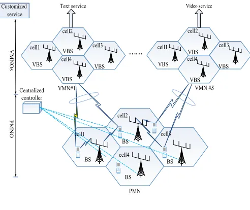
In this paper, we mainly study a multi-cell uplink VMIMO system including Nc cells, where each cell consists of one
BS equipped with Nr receiving antennas and Nu users with
single transmitting antenna. Besides, a centralized controller is required to determine the user grouping, resource allocation, and multi-cell information combining.
cell1 cell2
cell3
cell4 VBS
VBS
VBS
VBS
VMN#1
PMN Centralized
controller
cell1
cell2
cell3
cell4 BS
BS
BS
BS Customized
service
Text service
VMN #S
PMNO
VMNOs
Video service
cell1 cell2
cell3
cell4 VBS
VBS
VBS
[image:3.612.316.562.491.698.2]VBS
Fig. 1: Model of the WNV.
Further, the user schedulers in centralized controller selects
and the multi-cell joint processing is adopted at BSs side. Then, multiple user equipment in one group transmit the signal to all cells on the same RB, and the centralized controller combines the information received by different cells to further improve the system performance. The channel gain from the
u-th user of the j-th cell to the f-th antenna of the BS in the l-th cell is given by hf,l,u,j =
√
βf,l,u,jγf,l,u,j, where
γf,l,u,j is the small scale fading factor which is independent
and identically distributed zero mean, circularly-symmetric complex Gaussian CN(0,1) random variables, and βf,l,u,j is
the large scale fading coefficient which models the geometric attenuation and shadow fading that are assumed to be constant over a coherence time and known a priori.
In the WNV model, the network node such as a BS is partitioned into slices, and each of them represents a VMN respectively. As depicted in Figure 1, a physical mobile network (PMN) is split into SVMNs which support different users with different delay-bounded requirements.
As shown in Figure 2, let Ω={Ω1,· · · , Ωg,· · · , Ω|Ω|}
denote the set of user groups andγΩg denote the set of users
in user group Ωg. ThenγΩg corresponds to Nt mentioned
above. Further, assuming user group Ωg is scheduled in Mg
consecutive subcarriers with the first index pg, we write the
received signal vector of user groupΩgbefore MIMO detector
as
Yp,g=Hp,gXp,g+np,g, (1)
for p = pg, pg + 1, ..., pg +Mg −1, Mg = N g
RBN
RB
sc ,
where NRBg and NRB
sc denote the number of RBs occupied
by user group Ωg and the number of subcarriers in one RB
respectively, Hp,g is the NcNr×Nt virtual MIMO channel
matrix,Xp,gis theNt×1transmitting signal vector,np,gis the
NcNr×1 zero-mean additive white Gaussian noise (AWGN)
vector with covariance matrix E{np,gnp,gH
}
= σ2I NcNr.
Perfect power control over user groups is assumed in this paper. Thus, the total transmitting power of each user group signal vector Xp,g is constrained toEs, and the transmitting
power of each user signal is normalized to Es
Nt.
With the minimum mean square error (MMSE) frequency-domain equalization, the transmitting symbol vector can be estimated by
ˆ
Xp,g= (σ2INcNr+Hp,g
HH
p,g)−1Hp,gHYp,g, (2)
where σ2 denotes the spectral density power of noise. Then,
we get the post-processing SINR of user-u after MIMO equalization as [26]
SINRp,u= Es
σ2[(H
p,gHHp,g+σ
2
EsINt )−1]
u,u
−1. (3)
For uplink SC-FDMA systems, adjacent time-frequency RBs should be assigned to one user group. LetNRBdenote the
number of RBs, when the RB pattern contains only one RB, that is, only one RB is assigned to one user group, the number of RB pattern isNRB. When the RB pattern contains two RBs,
that is, two RBs are assigned to one user group, the number of RB pattern is NRB−1. In this way, when the RB pattern
contains NRB RBs, that is, NRB RBs are assigned to one
user group, the number of RB pattern is 1. Therefore, the total numberW of RB allocation patterns can be computed byW =
NRB+ (NRB−1) + (NRB−2) +· · ·+ 2 + 1 =
NRB(NRB+1)
2 ,
and the resource pattern matrixTcan be designed as follows:
pattern 1 2 · · · W
TNRB×W =
1 0 · · · 1 0 1 · · · 1
..
. ... . .. ...
0 0 · · · 1
RB1 RB2 .. .
RBNRB
, (4)
where RBn denotes the n-th RB, each element indicates
whether the RB is involved in the RB pattern (1) or not (0).
M1-DFT
M1-DFT
N-IFFT
N-IFFT
CP Insert
CP Insert
N-IFFT
N-IFFT
CP Insert CP Insert User group scheduling
M1-IDFT
M1-IDFT
N-FFT
N-FFT
CP Remove CP Remove Y 1 R
RNr
User Side BS1 cell cell 1 u i u j u K u 1 u i u j u K u 1 1 1 X T X Ti X Tj X T K MMSE ,: XT 1,: X TT j RB rb N RB 1 T 1 R B i RB 1 W T W
Centralized Controller and BSs Side Dynamic user grouping TT j RB rb N RB 1 T 1 R B i RB IDFT T M -T M-IDFT
T M T M DFT DFT -cell c N
cellNc
[image:4.612.313.564.231.555.2]Equalization BS c N Spatial, time-frequecy resource scheduling Statistical CSI
Fig. 2: Block diagram structure of VMIMO-SC-FDMA uplink system.
The available spatial resources come from the user grouping process. For the user group Ωg= (u1, u2,· · · , um), we can
write the group indexg ofΩg as [25], [26]
g=
m∑−1
j=1
∆j+ (um−um−1), m >1
u1 , m= 1
, (5)
where ∆j =
(
K−uj−1
m−j+ 1
) −
(
K−(uj−1)
m−j+ 1
)
,
{u1, u2,· · · , um} in group Ωg indicates the user index from
grouping matrix as follows:
B=
[
B(1),B(2),· · ·,B(K)
]
, (6)
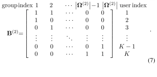
where B(k) denotes the fixed-k user grouping matrix. Then,
we take B(2) as an example, and it is designed as follows:
group index 1 2 · · · Ω(2)−1 Ω(2)user index
B(2)=
1 1 · · · 0 0
1 0 · · · 0 0
0 1 · · · 0 0
..
. ... . .. ... ...
0 0
0 0
· · · · · ·
0 1
1 1
1 2 3
.. .
K−1
K
.
(7)
B. The EB and QoS Exponent
Considering a queueing system with stationary ergodic arrival and service processes, the probability that the queue length exceeds a certain threshold C satisfies the following formula [17]:
− lim
C→∞
log (P{Q(∞)≥C})
C =θ, (8)
where P{a≥b} is the probability that a≥ b holds, Q(∞)
represents the steady-state queue length, θ is QoS exponent, which indicates the exponential decay rate of the QoS violation probability. A looser QoS requirement can be implied by a smaller θ, while a more stringent QoS requirement can be implied by a larger θ. θ → 0 means that there is no delay-bounded constraint, which represents that the system can tolerate unlimited long delay.
Based on the above concept of QoS exponent, the EB function, for a stationary ergodic traffic data arrival process
{A(t),t≥0}, can be described as follows:
EB(θ) =1
θtlim→∞ 1
tlogE [
eθA(t)
]
, (9)
whereA(t)represents the amount of arrival traffic data over the time interval[0, t).
In this paper, we make research in different scheduling peri-ods. Thus, optimization condition t→ ∞can be transformed into M Ts → ∞, i.e, M → ∞. Then, the EB function can
be accumulated by the amount of arrival traffic data in each scheduling period, and the equation can be written as follows:
EB(θ)=1
θMlim→∞ 1
M Ts logE
[
eθ[A1(Ts)+A2(Ts)+···+AM(Ts)] ]
, (10)
where Am(Ts) denotes the amount of traffic data in them
-th scheduling period. Because -the traffic flows in different scheduling periods are independent, the EB function can be simplified as:
EB(θ) =1θ lim
M→∞
1
M Tslog
{
E[eθA1(Ts)]· · ·E[eθAM(Ts)]}
= lim
M→∞
1 M
M
∑
m=1
g EBm(θ)
, (11)
whereEBgm(θ) = θT1slogE
[
eθAm(Ts)].
C. The EC of Sub-channel Based on FSMC Model
In this paper, we consider a RB as a sub-channel, which is comprised of consecutive NRB
sc subcarriers. Due to the
time-frequency correlation, we assume all subcarriers have the same channel state information (CSI) in one RB, which can be obtained by taking the average of the CSIs of the subcarriers within the RB. In addition, the received signal undergoes the flat Rayleigh fading in a typical sub-channel. To keep procedures simple, we drop the subscripts of subcarrier/RBs and groups in the description of this section.
Assuming that the channel state transfers L times in one scheduling period, as shown in Figure 3, one scheduling period
Tsconsists of Lframe slots Tp, that is, Ts=LTp.
Ă
s T p
T LTp
Ă
p lT
[image:5.612.52.303.125.249.2]2Tp
Fig. 3: The frame slots in one scheduling period.
For each sub-channel, VMIMO with Nt transmitting and
NcNr receiving antennas is used. We assume that the fading
gains between all antenna pairs are independent and identically distributed (i.i.d.) Rayleigh fading, and vary according to a Gauss-Markov model, which is widely adopted to describe the channel variation. Using this model, at time instancel, the channel matrix can be written as [22]
vec(H(l)) =√αvec(H(l−1)) +√1−αu(l), (12)
where 0 ≤ α ≤ 1, H(l) denotes the channel matrix of the l-th frame slot in one scheduling period, α is the channel de-correlation coefficient, which can be determined by αTc/(2Ts)=r
hh(Tc), where Tc is the channel coherence
time, rhh(t) denotes the time autocorrelation function. In
addition, u(l) ∈CNtNcNr×1 is independent with H(l−1).
u(l)andH(l)have i.i.d. complex GaussianCN(0,1)entries respectively.
In addition, let Γ = [Γ1,Γ2, . . . ,ΓQ+1] T
represent the thresholds of the element h of the matrix H in increasing order withΓ1= 0andΓQ+1=∞.his in stateqif the value
of h is between Γq and Γq+1. The value of h in state q is
denoted ashq, andhq = Γq.H can be designed as follows:
H=
h1,1 h1,2 · · · h1,Nt h2,1 h2,2 · · · h2,Nt
..
. ... . .. ...
hNcNr,1 hNcNr,2 · · · hNcNr,Nt
, (13)
wherehi,jdenotes the channel gain between thei-th receiving
antenna and the j-th transmitting antenna, and takes values from the set{hq|q= 1,2,· · · , Q}. Thus, we can get the state
space of matrixH, that isH∈{Hd|d= 1,2,· · ·, QNtNcNr
}
, whereHd denotes thed-th state of the matrixH. Specifically,
Hd is described as follows:
Hd =
hd1 hdNcNr+1 · · · hdNcNr(Nt−1)+1
hd2 hdNcNr+2 · · · hdNcNr(Nt−1)+2 ..
. ... . .. ...
where {hdγ|γ= 1,2,· · ·, NtNcNr }
takes values from
{hq|q= 1,2,· · ·, Q}.
When the initial state information in one scheduling period H(1) is given, and all elements of H(1) are h1, we can
compute the probability distribution ofH(2)according to Eq. (11). The specific equation can be designed as follows:
P(H(2)=Hd)=
∫hd1+1
hd1
fh(h1)dh∫hd2+1
hd2
fh(h1)dh· · ·∫
h
dNtNcNr+1
hdNtNcNr fh(h1)dh,
(15) where ∫abf(h)dh denotes the integral operation of the func-tionf(h)in the interval[a, b],fh(hq)denotes the probability
density function of hthat follows CN(√αhq,1−α).
In this way, we can get the probability distribu-tion of H in all frame slots in one scheduling period
{H(l)|l= 1,2,· · ·, L}.
Then, according to the Eq. (3), the capacity in thel-th frame slot using post-processing SNR can be expressed as [26]
rl=
∑
u∈Ωg
QNtNcNr∑
d=1 log2
Es
σ2[(H
dHHd+σ
2
EsINt
)−1]
u,u
P(H(l)=Hd).
(16) Further, the sub-channel capacity in one scheduling period can be written as follows:
R= (r1+···+rl···+rL)Tp
Ts
= (r1+· · ·+rl· · ·+rL)/L
. (17)
Under the condition of given H(1), we can get the sub-channel capacity in the 1st frame in one scheduling period
r1. Further, according to the nature of the Markov process,
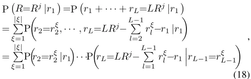
the probability distribution of the sub-channel capacity can be written as follows:
P(R=Rj|r 1
)
=P(r1+· · ·+rL=LRj|r1
)
=
|ξ|
∑
ξ=1 P
(
r2=r2ξ,· · ·, rL=LRj−
L∑−1
l=2
rξl−r1|r1
)
=
|ξ|
∑
ξ=1 P
( r2=r
ξ 2|r1
) · · ·P
(
rL=LRj− L∑−1
l=1
rlξ−r1rL−1=r ξ L−1
) ,
(18) where ξdenotes the number index of state combinations, |ξ|
denotes the total number of the combinations, rξl denotes the sub-channel capacity ofξ−thcombination in thel−thframe in one scheduling period and takes value from the capacity corresponding to all states. Therefore, under the condition of given initial channel state information, the average sub-carrier channel capacity in one scheduling period can be obtained as follows:
E [R] = J
∑
j=1
P(R=Rj|r1
)
Rj, (19)
where J denotes the number of channel capacity in the scheduling period.
As the dual concept of the EB source model, the EC is defined as the maximum constant arrival rate that a given channel service process can support in order to guarantee the QoS requirement specified by QoS exponent θ [16][32]. For a stationary ergodic service process,S(t)denotes the amount of data that the channel service counter can provide over the
time interval[0, t). Then,S(t) = ˜Rt, and the EC function can be designed as follows:
EC(θ) =−θ1 lim
t→∞
1 tlog E
[
e−θS(t)] = −1
θ tlim→∞ 1 tlog E
[
e−θRt˜ ] , (20)
whereR˜denotes the channel service rate over the time interval
[0, t).
Similar to the derivation process of EB function, the EC function can be rewritten as:
EC(θ)=−1
θMlim→∞ 1
M Ts logE
[
e−θ(R1Ts+R2Ts+···+RMTs) ]
, (21)
where Rm is the channel service rate in the m-th
schedul-ing period. Because the service rates in different schedulschedul-ing periods are independent, the EC function can be simplified as:
EC(θ)=−1θ lim
M→∞
1
M Ts
{
log[E(e−θR1Ts)· · ·E(e−θRMTs)]}
=− lim
M→∞
1 M
M
∑
m=1
g ECm(θ)
, (22)
where ECgm(θ) = −θT1
slogE (
e−θRmTs), andE(e−θRmTs)
= J
∑
j=1
P(R=Rj|r1
)
e−θRjTs.
Because we make research in each scheduling period, we drop the subscripts of scheduling period to keep description simple in the following.
D. Link Rate Virtualization and Instantiation
3GPP 5G network architecture will involve the integration of several cross-domain networks, and the 5G systems will be built to enable logical network slices across multiple domains. The proposal of this manuscript is implemented in radio access network (RAN) part and focuses on RAN slice. Advanced orchestration and management are required to release the configuration burden from users and enable an integrated end-to-end network slicing. The RAN part of 5G is significantly different from the core network (CN) and transport domains. It is difficult to virtualize RAN due to the diversity of wireless access technologies which are adapted to the random fading of wireless channels. The proposal provides a scheme of resource abstraction to hide the complex details of the fading channel. Thus, the main SDN principle of separating the control and user planes can also be adopted for the RAN. Moreover, the resource virtualization and instantiation algorithm proposed in this manuscript can be considered as the potential control plane function operated by the PMNO and VMNOs.
[image:6.612.52.301.441.520.2]Therefore, in this paper, we take the mean value of the link rates as its logic representation, that is, the virtual rate service of resources on the link. Correspondingly, EC, which is the actual rate service provided by the resources on the link, is considered as virtualization instance of the link rate.
resource reservation of VMNs with the delay-bounded QoS guarantee. On the other hand, to satisfy the delay-bounded QoS provisioning of traffic flows in each VMN with actual rate service, EC is used to provide the real service capability of the fading channel. Though these two processes may have a small rate gap, we can dynamically adjust the traffic flow access and the resource reservation to address the gap. The details are described below.
[ ]
ERm
Instantiate Instantiate
Resources reserved on one link Abstract (Specific delay-bounded QoS) Measure
[image:7.612.48.300.162.248.2]Actual service capability Virtual service rate
Fig. 4: Link rate virtualization and instantiation for them-th scheduling period.
E. Resource Abstraction Based on Gaussian-like Fitting Since the fading process that the signal undergoes is inde-pendent in each sub-channel, considering the complexity of analysing the probability distribution of the channel capacity, we give a Gaussian-like fitting method in the following.
Assuming that the Gaussian-like fitting curve Rb obeys
N(A, µ, σ2), which means that the probability density function
of Rb is Ae−
(Rb−µ)2 2σ2
, we give the optimization problem as follows:
mindEC−ECg (23)
subject to
J
∑
j=1
P(Rb=Rj)= 1, (23a)
whereP(Rb=Rj) =∫Rj+1
Rj e−
θRTˆ sAe−
( ˆR−µ)2
2σ2 dRˆ denotes the probability that Gaussian-like fitting capacityRbequalsRj, and
d
EC = −θT1
slog [
J
∑
j=1
∫Rj+1
Rj e−θ
ˆ
RTsAe−
( ˆR−µ)2 2σ2
dRˆ ]
denotes
the corresponding EC after the Gaussian-like fitting.
Further, we solve the above problem by the least squares fitting method, that is, we re-formulate the optimization problem (23) as
min J
∑
j=1
[ ∫Rj+1
Rj e−
θRTˆ sAe−
( ˆR−µ)2 2σ2
dRˆ−e−θRjTsP(R=Rj) ]2
.
Then, we obtain the optimal A,µandσ2.
Finally, after the Gaussian-like fitting process,ECd is close toECg, and it is computed by:
d EC=− 1
θTslog E
( e−θRTˆ s
)
=−θT1
slog (
∫+∞
−∞ e−θ
ˆ
RTsAe−
( ˆR−µ)2 2σ2 dRˆ
)
=ln 21 µ−θTsσ2
2 ln 2 −
log(2π)+2 log(Aσ) 2θTs
. (24)
From the above formula, it can be known thatECdis a linear function ofµ. In the resource virtualization phase, we compute
the virtual service rateE [R]with Gaussian-like fittingRb, that is,E [R]is equal toµ, thusECd is a linear function ofE [R]. Besides, because ECd is close to ECg, ECg is nearly a linear function of E [R].
IV. PROBLEM FORMULATION
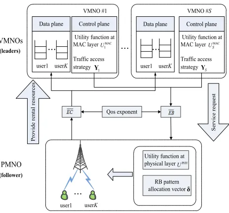
In this section, we consider the resource virtualization problem in the multi-cell wireless network virtualization en-vironment, where PMNO owns physical underlying resources and VMNOs provide flexible and customized services to end users by renting resources from PMNO. And we formulate the problem as a cross-layer Stackelberg game[27]-[31], where VMNOs are the players of the leader sub-game at the MAC layer and PMNO is the player of the follower sub-game at the physical layer respectively.
A. Optimization Scheme Using Stackelberg Game
In our model, {δ,Y} are the critical parameters in Stack-elberg game between PMNO and VMNOs, where δ is RB pattern allocation vector, and Y = [Y1,· · ·,Ys,· · ·,YS] is
traffic flow access matrix, whereYs is the traffic flow access
vector in the s-th VMN. Based on the duality and convex optimization theory, an iterative method is designed to obtain the optimal RB pattern allocation vectorδ∗=argmaxUPHY
Y
and the optimal traffic flow access vector in the s-th VMN Y∗s=argmaxUMAC
s δ, whereU
PHYis the utility function at the physical layer and UMAC
s is the utility function of the s-th
VMN at the MAC layer.
VMNOs
PMNO
Data plane
Utility function at MAC layer
Traffic access strategy
Control plane
user1 userK
VMNO #1
Data plane
Utility function at MAC layer
Traffic access strategy
Control plane
user1 userK
VMNO #S
Provide
rental
resources
Service
request
Utility function at physical layer
RB pattern allocation vector Qos exponent
user1 userK
(leaders)
(follower)
δ 1
Y YS
MAC 1
U MAC
S
U
PHY
[image:7.612.46.306.374.713.2]U
Fig. 5: The interaction diagram between PMNO and VMNOs.
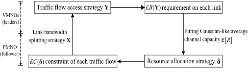
Figure 5 shows the leaders-follower dynamic interaction game between PMNO and VMNOs in one scheduling period. First, at the MAC layer, VMNOs set the traffic flow access strategy of each VMN{Y1,· · ·,Ys,· · ·,YS}, and present the
g
[image:7.612.327.559.425.641.2]user index 1 2 · · · u1 · · · um · · · K pattern index
E[R]gW×K =
0 0 · · · E [R1,g,u1] · · · E [R1,g,um] · · · 0
0 0 · · · E [R2,g,u1] · · · E [R2,g,um] · · · 0
..
. ... · · · ... · · · ... · · · ...
0 0 · · · E [RW,g,u1] · · · E [RW,g,um] · · · 0
1 2
.. .
W
. (25)
PMNO allocates the physical infrastructure resources to max-imize utility function UPHY at the physical layer according to the principle of on-demand allocation (ODA). Then, we can get the RB pattern allocation vector δ, the capacity of each link, and the correspondingECgconstraint of each traffic flow. Finally, VMNOs compete for these data rates of all links, which are from PMNO, adjust the traffic flow access strategy Y to maximize their utility function UMAC
s , update
the EBg requirements, and transfer the EBg requirements to the physical layer again. The above processes are repeated until VMNOs and PMNO achieve the balance of their own optimal strategy through the dynamic interaction. In this way, we can study an infinite number of scheduling periods, and get the EB requirement and EC constraint by taking the average of the EBg andECgin all scheduling periods.
B. Follower Side: The Resource Allocation Problem Model at The Physical Layer
In this section, we assume that the patternwcontainsv con-tinuous RBs, which is denoted as {RBwn|n= 1,2,· · · , v}.
Then, when the capacity that thew-th RB pattern is allocated to user-kin theg-th group in one scheduling period, the actual channel capacity can be denoted as Rw,g,k=Rw1,g,k+· · ·+
Rwv,g,k, whereRwv,g,k denotes the capacity of the wv-th RB
that is occupied by user-k in theg-th group.
However, obviously, it is very difficult to obtain and allocate
Rw,g,k in one scheduling period. This is because Rw,g,k has
a certain probability distribution as Eq. (18) rather than a certain value. Thus, in the following, we virtualize Rw,g,k to
E[Rw,g,k], which is considered as the virtual channel resource.
Further, according to the user grouping rule as Eq.(6), we can know that theg-th group includes user set {u1, u2,· · ·, um}.
Therefore, the virtual resource metric matrix in theg-th group can be expressed in (25), as shown at the top of this page.
Therefore, the total virtual resource metric matrix can be written as follows:
E[R]W×|Ω|×K=
[
E[R]1W×K E[R]2W×K · · ·
E[R]gW×K · · · E[R]|WΩ×|K
]
. (26)
DefineW|Ω|K×1 resource allocation vectorδ as δ=[δ1,1,1,· · ·, δ1,1,K,· · ·, δ1,|Ω|,1,· · ·, δ1,|Ω|,K,
· · ·, δW,|Ω|,1,· · ·, δW,|Ω|,K
] , (27)
whereδw,g,k is the assignment index which indicates whether
user-kin theg-th user group occupies thew-th RB pattern or not.
To provide service for more traffic flows, the resource allocation at the physical layer should meet the users’ traffic requirements as far as possible. In addition, considering the
proportional fairness among different users, we can design the utility function with ODA strategy at the physical layer as follows:
ODA:UODAPHY(δ) = K
∑
k=1 log
W
∑
w=1
|∑Ω|
g=1
E[Rw,g,k]δw,g,k
g EBk
, (28)
where EBgk is EBg requirement of user-k, which can be
obtained from the MAC layer, andδw,g,kis resource allocation
variable. Then, the resource allocation optimization problem at the physical layer can be designed as follows:
arg max
δ U
PHY
ODA(δ) (29)
subject to
AC1: A1δ= 1NRB×1; (29a)
AC2:
W
∑
w=1 K
∑
k=1
δw,g,k≥1 ∀g= 1,· · ·,|Ω|; (29b)
AC3: δw,g,k∈ {0, 1} ∀w= 1,· · · , W;
g= 1,· · · ,|Ω|;k= 1,· · · , K. (29c)
whereA1=TNRB×W ⊗11×K|Ω|. The constraint AC1 is to
ensure that each RB can only be allocated to one user group, AC2 is to ensure each user group can obtain one RB pattern, AC3 indicates whether the w-th RB allocation pattern is assigned to user-k in the g-th group (value 1) or not (value 0).
By solving problem (29), we can get the optimal RB pattern allocation resultδw,g,k∗, which means that the virtual resource,
that is the average channel capacity, has been allocated opti-mally. Then, we instantiate the virtual resource to ECg and derive theECg corresponding to traffic flow fs,k as follows:
g
ECfs,k = −
1
θfs,kTs
logE
[
e−θfs,kXfs,kRkTs ]
, (30)
wherefs,kis the requested traffic flows of thek-th user in the
s-th VMN,Xf
s,k is link bandwidth splitting variable of fs,k, θfs,k is the QoS exponent of fs,k, Rk is the capacity on the
k-th link, andRk= W
∑
w=1
|Ω|
∑
g=1
Rw,g,kδw,g,k∗.
MCA : UMCAPHY(δ) = K ∑ k=1 W ∑ w=1
|Ω|
∑
g=1
E [Rw,g,k]δw,g,k, (31)
ACA : UACAPHY(δ) = K/2
∑
i=1
∑
k∈Ω¯gi
E [Rw¯i,¯gi,k], (32)
where the user group set corresponding to the index
{
¯
g1,¯g2,· · ·,g¯K/2
}
is {(u1, u2),(u3, u4),· · ·, (uK, uK+1)} and the RB pattern set
corre-sponding to the index
{
¯
w1,w¯2,· · · ,w¯K/2
}
is
{(
RB1,· · · , RB2NRB/K )
, (
RB2NRB/K+1,· · · , RB4NRB/K )
, · · · ,
( RBN
RB−2NRB/K+1,· · ·, RBNRB )}
C. Leader Side: The Traffic Flow Access Problem Model at The MAC Layer
In this section, the traffic flow set
F={fs,k, s=1,· · ·,S, k= 1,· · ·,K} is given firstly. Then,
for ease of analysis, we assume that the arrival of traffic flow follows Poisson process. The QoS character of the traffic flow
fs,k can be described by
{ λf
s,k, D
max
s , P
out delay
}
, where λf s,k
is average arrival rate of fs,k, Dmaxs denotes the maximum
delay-bounded constraint of traffic flows in the s-th VMN,
Pdelayout is the delay-outage probability of fs,k, which shows
the probability that the delay exceeds a maximum delay bound. Then, based on the concept of Pdelayout in [17], we can get
Pdelayout =P{Delay≥Dmaxs }≈E[Rλfs,kYfs,k k]Xfs,ke
−θfs,kλfs,kYfs,kDsmax
, (33)
whereYf
s,kis the access variable of the traffic flowfs,k,E [Rk]
is the average capacity of user-k, θfs,k can be used for the
calculation of EB and EC, and the specific expression can be written as follows:
θfs,k ≈ −
1
λfs,kYfs,kD
max
s ln
[ Pout
delayE [Rk]Xfs,k
λfs,kYfs,k ]
. (34)
Further, for the given virtual link rate E [Rk], which has been determined by δ∗ at the physical layer, different VMNs compete with each other but have a consistent goal to max-imum the overall utility. Besides, considering the relevant contents in economics [33], we can design the overall utility function at the MAC layer as
UMAC= ∑S s=1
UMAC
s (Ys,Y−s)
= S
∑
s=1
[( α−β
K ∑ k=1 g EBf s,k )∑K
k=1
Yfs,kλfs,k
] , (35)
where UsMAC(Ys,Y−s) is the utility function of the s-th
VMN, Y−s is the set of traffic flow access vectors of all
VMNs, except the s-th one, α is the income of VMN, β
is the positive adjustment factor, EBgfs,k is EBg requirement
of fs,k, β K
∑
k=1
g EBf
s,k denotes the cost of the s-th VMN, α−β
K
∑
k=1
g EBf
s,kdenotes the unit profit in thes-th VMN [33].
Considering that a higher EB requirement delivers a better service, we setα=ρf(θfs,k
)
, whereρis the positive income coefficient and f(θfs,k
)
is the function positively related to
θfs,k.
Therefore, the traffic flow access and link bandwidth split-ting optimization problem at the MAC layer can be described as follows:
arg max
Y U
MAC (36)
subject to
BC1:Yfs,kλfs,k≤ECgfs,k ∀k= 1,· · ·,K;s=1,· · ·,S; (36a)
BC2:
S
∑
s=1
Xfs,k ≤1 ∀k= 1,· · ·,K; (36b)
BC3:0≤Xfs,k ≤1 ∀k= 1,· · ·,K;s=1,· · ·,S; (36c)
BC4:0≤Yfs,k ≤1 ∀k= 1,· · ·,K;s=1,· · ·,S.(36d)
The objective of the problem (36) is to maximize the utility function in thes-th VMN. BC1 guarantees the traffic flows that are admitted into VMNs are no more than the corresponding
g
ECconstraints, BC2 ensures the resources of all VMNs rented from each link must be no more than the total resource on the link, BC3 and BC4 are to ensure both Xfs,k andYfs,k value
from 0 to 1.
Further, by solving problem (36), we can get the traffic flow access variableYfs,k
∗. Then, theEBgrequirement of user-kat the physical layer can be written as follows:
g EBk=
S
∑
s=1
g
EBfs,k, (37)
where EBgfs,k is the EBg requirement of traffic flow fs,k,
and it has been assumed that the arrival of fs,k follows
Poisson process. Thus, the specific expression ofEBgfs,k can
be computed as follows:
g EBfs,k=
Yfs,k
∗λ
fs,k (
eθfs,k−1 )
θfs,k
. (38)
V. DYNAMIC ALGORITHM FOR RESOURCE VIRTUALIZATION PROBLEM
According to the different aims of PMNO and VMNOs, the wireless resource virtualization problem is decoupled into two sub-games, whose utility functions are both convex. Then, it can converge to the NE through multiple iterations. Further, a dynamic algorithm is developed, which includes the solution algorithms to the two sub-games and the message exchange between these dual processes.
A. Proposed Algorithm
To access and serve more traffic flows, we initializeYfs,k=1
andE [Rk] =N1
RB
N∑RB
n=1
|∑Ω|
g=1
E [Rn,g,k]. Then, according to the
Algorithm 1 Dynamic Algorithm for Resource Virtualization
Step 1: Initialize
{ λf
s,k, D
max s , Pdelayout
}
, Y(1)=1, X fs,k
(1) =
λfs,k
S
∑
s=1
λfs,k
,E[Rk] (1)
=N1
RB
N∑RB
n=1
|∑Ω|
g=1
E [Rn,g,k]andi= 0;
Step 2: Repeat
i⇐i+ 1; Computeθf(i)
s,k by Eq. (34);
ComputeEBgk(i)by Eq. (37);
Run Algorithm 2 for problem (29) to obtain δ(i) and E[Rk](i+1);
Update θ(i+1)f
s,k ,EBgfs,k
(i+1) andEBg
k(i+1) by Eq.
(34), Eq. (38) and Eq. (37) respectively;
Run Algorithm 3 for problem (36) to obtain Y(i+1);
Until Y(i+1)−Y(i)< ε
Step 3:
Obtain the optimal Y∗ =Y(i+1).
B. Solutions to the Sub-games
1) Resource Allocation Performed by PMNO
Obviously, the optimization problem (29) is a typical binary integer programming problem, and it is suitable to be solved by BNB algorithm [34]. However, BNB algorithm is too complex for a practical implementation especially when the number of users and RBs becomes large. Thus, inspired by the fast unfolding algorithm (FUA) [35] and the iterative Hungarian algorithm (IHA) [26], we propose an efficient algorithm including two parts. Specifically, we describe the detailed process as follows:
Part I: adopting the FUA to decompose the bipartite graph consisting of users and RBs into multiple sub-graphs based on the principle of maximizing network modularity
First, we introduce the concept of complete set, which consists of many complete subsets. In one complete subset, the intersection of all the elements must be empty, and the union of all the elements is the complete subset itself.
Second, because adjacent RBs must be assigned to one user group, we construct the complete RB pattern set by putting 0 or 1 on the underline of {RB1, , RB2, ,· · · , , RBNRB},
where putting 0 on the underline between RBi and RBi+1
means that RBi and RBi+1 are assigned to the same RB
pattern and vice versa. Then, it can be denoted as TRB =
{
TRB
1 ,· · · ,TRBt · · · ,TRB|TRB| }
, whereTRBis the number
of all subsets, andTRB= 2NRB−1.
Third, for all complete RB pattern subsets, we perform the same operation in the following. Specifically, we consider all possible matches between all users and RB patterns in the each subset as a bipartite graph. Then, after running the FUA, the bipartite graph is divided into multiple sub-graphs. Finally, we find out the subset that makes the modularity the most, the schematic is shown in Figure 6.
Part II: adopting the IHA to achieve the best match between user groups and RB patterns in each sub-graph
...
RB pattern 1 RB pattern 2 RB pattern N
FUA .. .
..
RB pattern 1 RB pattern 2 RB pattern N
user 1 user 2 user K
RB pattern n
RB pattern n+1
RB pattern N RB
pattern n RB pattern n+1
RB pattern N userj user j+1 user K
RB pattern 1
RB pattern 2
RB pattern m RB
pattern 1 RB pattern 2
RB pattern m user 1 user 2 user i
+
+
[image:10.612.316.566.58.205.2]
Fig. 6: The schematic of the FUA.
Assuming that there are V graphs, and one of sub-graphs contains M RB patterns and N users, similar to Eq.(6), we can generate all possible user groups as Ωˆ =
{
ˆ
Ω(1),· · ·,Ωˆ(n),· · ·, Ωˆ(N)}, where Ωˆ(n) denotes the user
group set includingnusers,Ωˆ(n)=Cn
N, andΩˆ= N
∑
i=1
Ci
N.
In addition, it is obvious that the indexm of M RB patterns can correspond to the indexwin RB pattern matrixT. Thus, according to Eq.(26), we can compute the metric matrixTPv
as
group index 1 2 · · · Ωˆ RB pattern index
TPv=
U1,1 U1,2 · · · U1,|Ωˆ|
U2,1 U2,2 · · · U2,|Ωˆ|
..
. ... . .. ...
UM,1 UM,2 · · · UM,|Ωˆ|
1 2
.. .
M
,
(39) where Um,g =
∑
k∈Ωg
log
(
E[Rm,g,k]
g
EBk
)
, E[Rm,g,k] can
corre-spond to E[Rw,g,k] in Eq.(26).
The specific steps can be described as follows:
Algorithm 2 Resource reservation algorithm based on fast unfolding and iterative Hungarian method
Step 1:
Initialize t= 0 andv= 0; Step 2:
Generate the complete RB pattern set by putting 0 or 1 on the underline of{RB1, , RB2, ,· · ·, , RBNRB}
as mentioned above; Repeat
t⇐t+ 1;
Consider all possible matches between all users and RB patterns in thet-th subset as a bipartite graph; Run the FUA to decompose the bipartite graph into multiple sub-graphs;
Compute the corresponding modularity; Until t= 2NRB−1
Step 3: Repeat
v⇐v+ 1; Repeat
Compute the metric matrix TPv by Eq. (39);
Select the maximum value U∗=Um∗,g∗ from
matrix TPv, and(m∗, g∗) = arg max
m,g {
Um,g|
m∈[1, M], g∈[1,Ωˆ]};
Delete the m∗-th row and theg∗-th column in matrix TPv;
Record the row labels of elements whose values are 1 in theg∗-th column of matrix B;
Traverse all the elements of the row, record the column labels of elements whose values are 1; Delete the corresponding columns in matrix TPv;
Until TPv=ϕ
Until v=V
Record the corresponding δ.
2) Traffic Flow Access Control Performed by VMNOs The optimization problem (36) is a nonlinear programming problem with high complexity, which involves the traffic flow access variable Yfs,k and link bandwidth splitting variable Xfs,k. To make it tractable, we propose a dynamic iteration
method including two steps. The first step is to computeXfs,k
based on Yfs,k obtained by the last iteration, and the second
step is to get the optimal Yfs,k based on the results of step1.
The specific update process is designed as follows:
First, we introduce the Lagrangian factor ωfs,k ≥ 0 to
the optimization problem (36). Then, the problem (36) is re-formulated in Lagrangian form as:
LMAC= S
∑
s=1
[( α−β
K
∑
k=1
g EBfs,k
)∑K
k=1
Yfs,kλfs,k ]
+ K
∑
k=1
ωfs,k (
g
ECfs,k−Yfs,kλfs,k
) . (40)
It is noticed that the following conditions aboutωfs,k must
be satisfied:
0≤ωfs,k⊥ (
g
ECfs,k−Yfs,kλfs,k )
≥0, (41)
where the notation 0≤a⊥b≥0 meansa·b= 0,a≥0and
b≥0. The iterative formula of ωfs,k is described as follows:
ωfs,k(t+ 1) = [
ωfs,k(t) +∇ωfs,k (
Yfs,kλfs,k−ECgfs,k )]+
, (42)
where (•)+ = max(•,0), t is the iteration index, ∇ωfs,k is
the positive iteration step.
Second, for given Yfs,k, we analyze the characteristics of
Eq. (40). Take the derivative of Eq. (40) with respect toXfs,k
as follows:
∂LMAC
∂Xfs,k
=ωfs,k
E
[
Rke−Xfs,kθfs,kTsRk
]
E
[
e−Xfs,kθfs,kTsRk
] . (43)
Obviously, ∂L∂XMAC
fs,k > 0, which denotes Eq.(40) is
mono-tonically increasing with respect toXfs,k. Then,Xfs,k can be
updated by the gradient of the utility function, and the specific iterative equation can be written as:
Xfs,k(j+1) =Xfs,k(j) +dfs,k
∂LMAC
∂Xfs,k
Xfs,k=Xfs,k(j)
, (44)
wherej is the iterative index, anddfs,k indicates the strategy
adjustment step size, which is used to control the speed of strategy adjustment.
Third, derive the first derivative of LMAC with respect to
Yfs,k as follows:
∂LMAC
∂Yfs,k =
( α−β
K
∑
k=1
Yfs,kλfs,k(eθfs,k−1)
θfs,k
) λfs,k
−βλfs,k
(
eθfs,k−1) θfs,k
K
∑
k=1
Yfs,kλfs,k −ωfs,kλfs,k
. (45)
Then, derive the second derivative of LMACwith respect to
Yfs,k as follows:
∂2LMAC
∂Yf s,k
2 =−2β
λ2 fs,k
(
eθfs,k −1 )
θfs,k
. (46)
It is obvious that ∂∂Y2LMAC
fs,k2
<0 . Thus, LMAC is a convex
function with respect to Yfs,k. To obtain the optimal utility
function value and traffic flow access rate, we use the gradient iteration method to compute the extreme point of Eq. (40). The specific iterative equation is as follows:
Yfs,k(τ+1) =Yfs,k(τ) +υfs,k
∂LMAC
∂Yfs,k
Yfs,k=Yfs,k(τ)
, (47)
whereτ is the iterative index, and υfs,k indicates the strategy
adjustment step size.
The specific algorithm is described as follows:
Algorithm 3 Gradient Iteration Algorithm for Traffic Flow Access Control
Step 1:
Initializewfs,k,dfs,k,κ= 0,Yfs,k(1) = 1,Xˆfs,k(0) = 0
andYˆfs,k(0) = 0;
Step 2: Repeat
κ⇐κ+ 1; Step 2a:
Initialize j= 0andXfs,k(1) = 0;
Repeat
j⇐j+ 1;
UpdateXfs,k(j+1) by Eq.(44);
Until
S
∑
s=1
Xfs,k≥1
ˆ
Xfs,k(κ)⇐Xfs,k(j+ 1);
Step 2b: