Maximum Achievable Sum Rate in Highly
Dynamic Licensed Shared Access
Samuel Onidare, Keivan Navaie, Qiang Ni
School of Computing and Communications, InfoLab21 Lancaster University, Lancaster, United Kingdom, LA1 4WAAbstract—In this paper, we consider a power allocation scheme that maximizes the sum spectral efficiency of the licensee in a dynamic Licensed Shared Access (LSA) system. In particular, our focus is on the time intervals in which the incumbent system is active in the spectrum. We derive an expression for the interference distribution of the licensee, e.g., a mobile network operator, utilizing a spectrum belonging to an airport incumbent under the LSA spectrum sharing. Formulating an optimization problem to maximize the sum spectrum efficiency subject to the interference threshold constraint at the licensee, we then show its convexity, and obtain its optimal solutions. We further investigate the impact of sum rate maximization on the fairness of network resource allocations. Simulation results show a significant gain in the achievable spectrum efficiency, especially during the intervals in which the incumbent system is active in the LSA band. This paper provides quantitative insights on the maximum achievable sum rate in an LSA system in which both the licensee and the incumbent systems are active at the same time.
Index Terms—Airport Traffic Control; Dynamic Spectrum Sharing;Licensed Shared Access; Sum rate.
I. INTRODUCTION
Licensed Shared Access (LSA) is a dynamic spectrum sharing (DSS) scheme proposed to address the challenges posed by the exponential growth in bandwidth demand [1]. A fundamental feature of the original LSA scheme is a static exclusion zone, which could cover a wide geographical area, up to 25 km radius, if the incumbent is an airport [2]. Having a static exclusion zone results in a significantly large swath of spatial spectrum hole. Spectrum usage can be enhanced by introducing a dynamic exclusion zone.
Addressing this issue, the dynamic form of LSA is pro-posed by the European Union (EU) regulatory framework in [3]. Algorithms for spectrum allocation in dynamic LSA are developed in [4]–[6]. In [7] spectrum resource allocation in the cellular band between a cellular network and an LSA system is investigated, and a system model based on homogenous queues is used to analyse the performance. Queueing theory is also used in [8] to model the LSA operation. The authors of [9] presented experimental evaluations of dynamic LSA operation in an LTE testbed. Furthermore, the impact of dynamic nature of the incumbent (airport) telemetry traffic together with the primary cellular network traffic is modelled in [10] using non-homogeneous queues.
The performance of primary cellular network is also directly affected by the aircrafts’ flight path as it is investigated in
[11]. To analyse this effect, [11] employs two different path-loss models including two-ray ground reflection and free space path loss to represent the communication behavior of the two system sharing the spectrum. In [12], the horizontal form of the LSA spectrum sharing between a macro and a micro cellular networks owned by two operators is presented. In this scenario the licensee is the micro cellular network and the macro cellular network is the incumbent.
At a given time instant, telemetry communication between the airport traffic control (ATC) and the flying airplane only affects the cellular users and/or being affected by the cellular user within a small portion of the exclusion zone. Furthermore, above a certain altitude the path-loss experienced by the licensee system’s transmitted signal only results in a negligible level of interference at the aircraft. In cases where the aircraft is interfered by the licensee system, the power transmission by the licensee nodes can be accordingly adjusted to sufficiently reduce the interference level.
On the basis of this, the authors in [2] modelled and demon-strated the feasibility of a highly dynamic LSA under three possible transmit power regimes. The performance evaluation in [2] is solely based on simulations and they fail to provide analytical insights on the important aspects of the system design. The authors of [13] obtained the experienced reduction of the achieved data rate in the licensee system as a result of reducing the transmit power in the licensee system.
As it is seen, most of the previous works on the LSA are either focused on modeling the spectrum utilisation for a given setting, see, e.g., [8], [10], [13], or evaluate performance met-rics such as the interruption probability, blocking probability, average number of connected users, service failure, mean bit rate, etc [7], [8], [10], [13]. In contrast with the previous works, here our main objective is to explore techniques for optimizing the system spectrum efficiency, especially during the time intervals in which the LSA band is not available while ensuring the allowable interference threshold is not exceeded.
II. SYSTEMMODEL
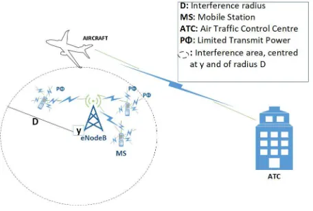
Fig. 1. The system model.
is communicating with the aircraft(s) during and shortly after take-off as well as before and during landing. When the incumbent system is active the spectrum can be said to be busy, occupied, or unavailable. At other times, the spectrum is free and available for the MNO unrestricted access. During the non availability of the spectrum, the licensee transmit power, and by implication the system’s capacity [14], becomes constrained by the allowable interference power that the in-cumbents system can tolerate, i.e., the system’s interference threshold. In other words, for a fixed transmit power, the total interference must be kept below a certain value.
A. The Interference
We focus on the interference that could impair the ATC transmission to the flying aircraft during the take-off or landing. Premised on the assumption that the eNodeB or base station antenna height is sufficiently low relative to the ATC tower with a directional pattern (directed downwards to the mobile stations), the omni-directional transmissions of the mobile stations (MSs) become the main components of the interfering signal [2].
The spatial distribution of the MSs in the cell is represented by a Poisson point process,
ϕ={k1, k2, ...kN}. (1)
The interference to a given aircraft located at a point in the vicinity of the cellular network is
X
k∈ϕ
Pkhkl(ky−kk), (2)
where, l(k) = kkk−α, α is the path loss exponent, h
k the
fading coefficient which is an exponential random variable, i.i.d for k∈ϕ with E[h] = 1, Pk is the MS transmission
power, l is the distance related power loss, and k denotes individual nodes or MSs randomly located in licensee’s cells. We then define distanceky−kk,(k∈ϕ), askrk ≤Dand the intervening area between them can then be represented as a ballb(y, D),centred atyand of radiusD. Therefore, we can define an interference point processϕI =ϕ∩b(y, D), (similar
to the inner city model of the Cox process), where ϕI, and
ϕare Poisson processes with densityλI, andλ, respectively,
andλI =λcddrd−1, where,cd=kb(0,1)k is the volume of
d-dimensional unit hyper ball.
The total interference power measured at the origin, i.e. the location of the aircraft from MSs located within distance D
can then be characterized as
ID=
X
r∈ϕI
l(r), (3)
For brevity we assume thatl(r)is monotonically decreasing,
limr→0l(r) = ∞ and limr→∞l(r) = 0. Similar to the
approach in [15], here we need to obtain the cumulative distribution function (CDF) of the interference power,ID.
FID(ω) =E(expjωID), (4)
whereF(.)andE(.)are the Fourier transform, and expectation operators, respectively. Considering that there are expectedK
nodes within ballb(y, D), we write
FID(ω) =E(E(expjωID|k))
=
∞
X
k=0
exp−λIπD2(λ
IπD2)k
k! E(exp
jωID|k). (5)
We further note that the nodes are independent and identically distributed (i.i.d) within ballb(y, D), with radial density of
fR(r) =
2r
D2, 0≤r≤D,
0, otherwise. (6)
The interference,ID, is the summation of independent random
variables, thenE(expjωID|k)can be expressed as;
E(expjωID|k) = [E(expjωl(r))]k,
=
Z D
0
2r
D2exp
jωl(r)dr
k
.
(7)
Combining (5) and (7), setting D → ∞, r(x) =l−1(x), and applying the standard path loss modell(r) =r−α, we have:
FI(ω) = exp
jλIπω
Z ∞
0
x−α2 expjωxdx
. (8)
In practice,α≥2, then (8), is further simplified as
FI(ω) = exp
−λIπΓ(1−β) exp−
πβ 2 ωβ
, ω≥0, (9)
where β = α2, Γ(.) is the gamma function and we note
FI∗(−ω) = FI(ω). Using the approach in [15], the
proba-bility density function (PDF) of (9) is then estimated as an infinite series. Taking its inverse Fourier transform, we have,
fI(i;β) = 1
πi
∞
X
k=1
Γ(βk+ 1)
k!
λIπΓ(1−β)
iβ
k
sinkπ(1−β),
(10) and the CDF is
FI(i;β) = 1
π
∞
X
k=1
Γ(βk)
k!
ρ
iβ
k
sinkπ(1−β), (11)
B. Achievable Sum Rate
In cases where the incumbent system is not utilizing its spectrum, the licensee eNodeB is able to transmit at maximum power to guarantee the desired signal to noise and interference ratio (SINR) for each MS according to its QoS requirement. The achievable bit rate for each channel isC=1
2log2(1 +γ),
whereγ is the SINR.
In our model, the users are assumed to be randomly dis-tributed according to (6) within the cell. We thus represent the channels for k users as a vector of random variables,
H = [H1...HK]T, and correspondingly the eNodeB
down-link transmit-signal vector as X = [X1...XK]. Therefore,
the received signal power for kusers, P = [P1...PK]T, is
P =XH+Z and
γ= XH+Z
Z =
P
Z, (12)
where Z is the additive white Gaussian noise vector, (Z = [Z1...ZK]T), assuming no additional interference.
Further-more,Hk= rGα k
(G, is a propagation constant), and achievable sum rateCsum is:
Csum= K
X
k=1
1
2log2
1 +XkHk+Zk
Zk
. (13)
III. MAXIMIZING THEACHIEVABLESUMRATE
If the LSA spectrum is unavailable, the eNodeB has to limit its transmit-power to ensure that the total interference power of the licensee (the MNO) does not exceed the interference threshold. In other words, the transmit power should be reduced such that the outage probability, (1− Ps(θ)), of
the incumbent network does not exceed a given performance thresholdθ, wherePs(θ) =P(SIN R > θ)is the transmission success probability. Thus while maximizing the achievable sum capacity, the sum transmit power of the eNodeB must be such that the total interference caused to the incumbent does not cause outage. Maximization of the sum rate is then formulated as the following:
Csum∗ = max
(P)
K
X
k=1
1
2log2
1 + XkHk+Zk
Zk
, (14)
s.t.
E(P)
1
π
K
X
k=1
Γ(βk)
k!
ρ
iβ
k
sinkπ(1−β)≤Ith. (15)
In this optimization problem, (15), is the constraint on the system’s total interference. On the left-hand side of (15),E(P) is the expected value of all the MSs received power while the second term FI(i;β), is the CDF of the system interference
(see, (11), Ith is the maximum allowed interference for
in-cumbents safe operation. The constraint placed on the eNodeB transmit power by (15) is such that,
K
X
k=1
XkHk+Zk=E(P)1
π
K
X
k=1
Γ(βk)
k!
ρ
ıβ
k
sinkπ(1−β).
(16)
A. Optimal Power Allocation
Proposition:The optimization in (14) is a convex optimization problem.
Proof: By substituting (16) into (14) the objective function becomes:
Csum∗
= max (Pk)
K
X
k=1 1
2log2 1 +
Pkπ1Γ(kβk!)
ρ iβ
k
sinkπ(1−β)
Zk
!
.
(17)
The Hessian of the objective function is:
δ2C∗
sum
δPk2
=
−
Γ(βk)
πk!
ρ iβ
k
sinkπ(1−β)
2
2λln(2)(Zk)2
"
1
1 +Pk
Γ(βk) πk!
ρ iβ
k
sinkπ(1−β)
Zk
2 #
,
(18)
which is non-positive for all values ofPk, hence the
optimiza-tion objective funcoptimiza-tion is concave.
In order to solve (14), the sum constraint on the transmit power must be decoupled. This is done by introducing a new set of variables[Ith1, . . .]. Using Lagrangian method, the
corresponding Lagrangian is
L(Pk, λ) =
max
(Pk)
K
X
k=1
1
2log2 1 +
Pk1π
Γ(βk)
k!
ρ
θβ
k
sinkπ(1−β)
Zk
!
,
−λ 1
π
K
X
k=1
PkΓ(βk)
k!
ρ
θβ
k
sinkπ(1−β)−Ithk
!
.
(19)
Karush Kuhn Tucker conditions are:
δL
δPk =
= 0 ifPk >0,
≤0 ifPk = 0.
(20)
Setting δPδL
k = 0 gives
Φk
2λln(2)Zk
" QK
j6=k
1 + PiΦj
Zj
1 + PkΦk
Zk
QK
j6=k
1 +PiΦj
Zj
#
(21)
whereΦk=
Γ(βk)
πk!
ρ iβ
k
sinkπ(1−β). Therefore, the optimal allocated powerPk∗ is
Pk∗= 1 Φk
"
1
2λln(2)−Zk
#
. (22)
IV. SIMULATIONRESULTS ANDANALYSIS
Here, we assume an average maximum transmit power
0.2 0.3 0.4 0.5 0.6 0.7 0.8 0.9 Limit Power Level (%tage of Max Transmit Power) 3.2
3.4 3.6 3.8 4 4.2 4.4 4.6
SE (b/s/Hz)
[image:4.612.343.527.57.203.2]optimized Sum capacity normal Sum capacity
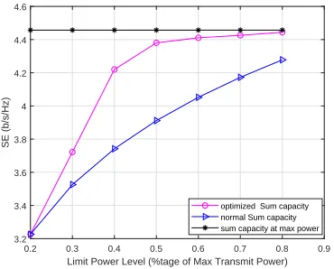
Fig. 2. Csum∗ , and normal sum rate vs. limit power level.
0.2 0.3 0.4 0.5 0.6 0.7 0.8 0.9 Limit Power Level (%tage of Max Transmit Power) 3.2
3.4 3.6 3.8 4 4.2 4.4 4.6
SE (b/s/Hz)
optimized Sum capacity normal Sum capacity sum capacity at max power
Fig. 3. ComparingC∗
sumwith the achievable sum rate at max. power.
thus the licensee transmit power has to be reduced to prevent harmful interference to the incumbents communication.
We also investigate different scenarios of limiting transmit power as a result of the incumbents ATC transmission. Here, we look at the cases with limited power, 20% -80% of the maximum average transmit power. An increase is seen in the spectrum efficiency when achievable sum rate is optimized. Furthermore, while the curve of the achievable sum rate with-out optimization increases linearly with increase in transmit power (during the limited power regime), the curve of the optimized sum rate tends to increase exponentially with the increase rate is reduced by increasing the power.
At the lower limited transmit power, there is not much gain achieved when the sum rate is optimized. In fact, at 20% of the average maximum transmit power, the sum capacity optimized value is almost the same as the non-optimized value. However, as the power level increases, the marginal gain with optimization also increases. The rate of increase differs between successive level reaching its peak at the 40% mark, from where the slope of the rate of increase gradually reduces as the limit power tends to average maximum power, when spectrum becomes available again.
In Fig. 3, we plot the achievable sum rate at maximum
1 2 3 4 5
User index 0
0.5 1 1.5 2 2.5 3 3.5
SNR
104
[image:4.612.80.264.60.206.2]optimized sum rate normal sum rate
Fig. 4. SNR of the individual usersCsum∗ vs. normal sum rate.
1 2 3 4 5
User index 0
2 4 6 8
SNR
106
optimized sum rate normal sum rate
1 2 3 4 5
User index 0
2 4 6 8 10
SNR
106
optimized sum rate normal sum rate
1 2 3 4 5
User index 0
2 4 6 8 10
SNR
106
optimized sum rate normal sum rate
1 2 3 4 5
User index 0
2 4 6 8 10
SNR
106
[image:4.612.80.265.251.400.2]optimized sum rate normal sum rate
Fig. 5. SNR distribution for different transmit power limits.
transmit power, i.e., when the spectrum is free of incumbents transmission and hence licensee can operate without the re-striction imposed by the allowed interference threshold. A comparison of this with the proposed maximized sum rate shows the significance of adopting a sum rate maximization power allocation during periods of unavailability of the LSA band. From the 50% mark onwards, the difference between the sum rates at maximum transmit power and the optimized limit power becomes significantly smaller and eroded. The implication of this is that, if the transmit power reduction during the incumbent occupation of the spectrum is a few percentages lower than the actual transmit power when the spectrum is vacant (about 20-30% lower), the licensee network can still operate at an almost similar aggregate quality of service (QoS) for its users.
[image:4.612.340.558.252.370.2]It can be argued that a situation where some of the users actually suffered outage or low SNR value at the expense of total network sum rate optimization, while some other users have very high SNR value is not ideal, or does not reflect well on the network performance. To the contrary, in the light of todays and future networks heterogeneity and the possible coexistence of an LSA system with the primary or main cellular network, the observed disparity in the SNR values can be leveraged upon to provide an improved joint spectrum efficiency of the licensee main cellular band and the LSA band. Fig. 5, shows the SNR variation at different limit power (20%, 40%, 60% and 80% of average maximum transmit power) levels for five users. It is interesting to note that in each of the graphs, an increase in the power level does not necessarily lead to increase in the SNR fairness among users, i.e., to say, the disparity in the committed network resources did not decrease even at higher power level. Similar trend is observed for 3 and 4 users. In fact, Fig. 5, for 5 users, indicate less outage ratio at the 40% and 60% limited power, than at the lower and higher power level. This is consistent with Fig. 2 and 3 where higher marginal gain in spectrum efficiency is recorded in the mid-region than at the extreme boundaries (20% and 80%) of the power limit range.
V. CONCLUSION
We proposed a technique for maximization of the sum rate of an MNO licensee under the dynamic LSA spectrum sharing scheme with an airport incumbent during periods of nonavailability of the LSA band, i.e. when the incumbent is using the spectrum for its ATC transmissions. Our simulations results show that maximizing the system spectrum efficiency comes at a cost to users’ fairness. However, considering the fact that todays, and to a larger degree, next-generation network is highly diversified and heterogeneous in nature, the trade-off between system SE and fairness to individual users could be an advantage rather than a disadvantage. This is more so, considering the fact that users close to the MNO cell centre could be afforded higher SNR while their contribution to the total interference experienced by the incumbent operation is minimal compared to the users closer to the cell edge.
VI. ACKNOWLEDGMENT
The work of Samuel Onidare is supported by the National Information Technology Development (NITDA), under the Federal Ministry of Communication Technology, Federal Re-public of Nigeria. In addition, the research in this paper was also partly supported by H2020-MSCA-RISE-2015 ATOM 690750.
REFERENCES
[1] Ericsson, “ericsson mobility report,” June, Tech. Rep., 2017.
[2] A. Ponomarenko-Timofeev, et. al, “Highly Dynamic Spectrum Man-agement within Licensed Shared Access Regulatory Framework,”IEEE Communications Magazine, vol. 54, no. 3, pp. 100–109, March 2016. [3] Fp7 project adel. [Online]. Available: http://www.fp7-adel.eu
[4] V. Frascolla, et. al, “Dynamic Licensed Shared Access - A New Architecture and Spectrum Allocation Techniques,” in2016 IEEE 84th Vehicular Technology Conference (VTC-Fall), Sept 2016, pp. 1–5.
[5] Q. Ni and C. C. Zarakovitis, “Nash Bargaining Game Theoretic Scheduling for Joint Channel and Power Allocation in Cognitive Radio Systems,”IEEE Journal on Selected Areas in Communications, vol. 30, no. 1, pp. 70–81, January 2012.
[6] A. Al-Dulaimiet. al, “Adaptive Management of Cognitive Radio Net-works Employing Femtocells,” IEEE Systems Journal, vol. 11, no. 4, pp. 2687–2698, Dec 2017.
[7] I. Gudkova,et. al, “Service Failure and Interruption Probability Analysis for Licensed Shared Access Regulatory Framework,” in2015 ICUMT, Oct 2015, pp. 123–131.
[8] V. Y. Borodakiy,et. al, “Modeling Unreliable LSA Operation in 3GPP LTE Cellular Networks,” in 2014 6th International Congress on Ul-tra Modern Telecommunications and Control Systems and Workshops (ICUMT), Oct 2014, pp. 390–396.
[9] P. Masek,et. al, “Experimental Evaluation of Dynamic Licensed Shared Access Operation in Live 3GPP LTE System,” in 2016 IEEE Global Communications Conference (GLOBECOM), Dec 2016, pp. 1–6. [10] I. Gudkova,et. al, “Modeling and Analyzing Licensed Shared Access
Operation for 5G Network as an Inhomogeneous Queue with Catastro-phes,” in2016 ICUMT, Oct 2016, pp. 282–287.
[11] E. V. Mokrov and I. A. Gudkova, “Performance Evaluation of Dynamic Licensed Shared Access Operation through a Model of a Stand-Alone Cell,” inPeoples Friendship University of Russia, Oct 2016, pp. 35–41. [12] M. Hafeez and J. M. H. Elmirghani, “Green Licensed-Shared Access,” IEEE Journal on Selected Areas in Communications, vol. 33, no. 12, pp. 2579–2595, Dec 2015.
[13] I. Gudkova,et. al, “Modeling the Utilization of a Multi-tenant band in 3GPP LTE System with Licensed Shared Access,” in2016 ICUMT, Oct 2016, pp. 119–123.
[14] M. G. Khoshkholgh,et. al, “Access Strategies for Spectrum Sharing in Fading Environment: Overlay, Underlay, and Mixed,”IEEE Transactions on Mobile Computing, vol. 9, no. 12, pp. 1780–1793, Dec 2010. [15] E. S. Sousa and J. A. Silvester, “Optimum Transmission Ranges in