Bayesian Prediction based on an Adaptive Type II Progressive Censored Data from the Generalized Exponential Distribution

(1)

Bayesian Prediction based on an Adaptive Type-II

Progressive Censored Data from the Generalized

Exponential Distribution

M. M. Mohie El-Din

Department of Mathematics Faculty of Science Al-Azhar University

Egypt

M. M. Amein

Department of Mathematics Faculty of Science Al-Azhar University

Egypt

A. R. Shafay

Department of Mathematics Faculty of Science Fayoum University

Egypt

S. Mohamed

Department of Mathematics Faculty of Science Fayoum University

Egypt

ABSTRACT

In this paper, based on an observed adaptive Type-II progressively censored sample from the generalized exponential distribution, the problem of predicting the order statistics from a future unobserved sample from the same distribution is discussed. The description of the model of the adaptive Type-II progressively censored sample from the generalized exponential distribution is presented. Also, Markov chain Monte Carlo method is applied to construct the Bayesian prediction intervals of the order statistics from a future sample from the same distribution. Finally, results from simulation studies assessing the performance of our proposed method are in-cluded and then an illustrative example using real data set is pre-sented for illustrating all the inferential procedures developed here.

General Terms

AMS 2000 Subject Classification: Primary 62G30; Secondary 62F15

Keywords

Adaptive Type-II progressive censored scheme, Bayesian predic-tion, Generalized exponential distribupredic-tion, Markov chain Monte Carlo technique

1. INTRODUCTION

There are several types on life testing in which units are removed or lost from the experiment before the failure. Data which obtained from such experiment are called censored data. The most common reason for censoring is reducing the total time of the test and the associated cost and effort. Also, a censoring scheme which can bal-ance between, total time spent for the experiment, number of units placed on the experiment and the efficiency of statistical inference based on the results of the experiment, is desirable.

Type-I (time) and Type-II (failure) censoring schemes are the most common censoring schemes. Under Type-I censoring scheme, the life testing experiment will be stopped at a pre-fixed timeT, while under Type-II censoring scheme, the life testing experiment will be terminated at the time when therth_{failure is observed.} Pro-gressive Type-II censoring scheme is a generalization of Type-II

censoring scheme, wherenunits are placed on the life testing ex-periment and onlymfailures are going to be observed. At the first observed failure,R1 of the surviving units are randomly selected and removed. When the second failure is observed,R2of the sur-viving units are randomly selected and removed. The experiment will be terminated at when themth_{failure is observed and all} re-mainingRm=n−R1−R2−...−Rm−1−msurviving units are removed. We denote a progressively Type-II censored sample byX1:m:n< X2:m:n < ... < Xm:m:n. For extensive reviews of the literature on progressive censoring, readers may refer to Balakr-ishnan and Aggarwala (2000), BalakrBalakr-ishnan (2007), Ng and Chan (2007), and Mohie El-Din and Shafay (2013).

Recently, Ng et al (2009) have suggested an adaptive Type-II gressive censoring which is a mixture of Type-I and Type-II pro-gressive censoring schemes. In this censoring scheme, we allow

R1−R2− · · · −Rmto depend on the failure times so that the

effective sample size is alwaysm which is fixed in advance. A properly planned adaptive progressively censored life testing ex-periment can save both the total test time and the cost induced by failure of the units and increase the efficiency of statistical analy-sis. This censoring scheme can be described as follows: Consider nidentical units under observation in a life-testing experiment and suppose the experimenter provides a timeT, which is an ideal to-tal test time, but we may allow the experiment to run over timeT. If themth_{progressively censored observed failure occurs before} timeT (i.e.Xm:m:n< T), the experiment terminates at the time Xm:m:n(progressive Type-II censoring case); see Fig. 1.

Otherwise, once the experimental time passes timeTbut the num-ber of observed failures has not reachedm, we would want to ter-minate the experiment as soon as possible. Therefore, we should leave as many surviving items on the test as possible. SupposeJ is the number of failures observed before timeT, i.e.XJ:m:n <

T < XJ+1:m:n, J = 0,1, ..., m, where X0:m:n ≡ 0 and

Xm+1:m:n ≡ ∞. After the experiment passed timeT, we set

RJ+1 = ... =Rm−1 = 0andRm =n−m−

PJ

i=1Ri; see

Fig.2.

This formulation leads us to terminate the experiment as soon as possible if the (J + 1)th _{failure time is greater than} _T _for

J+ 1 < m. The value of T plays an important role in the

(2)

[image:2.595.316.564.425.533.2]

Fig. 1. experiment terminate before timeT.

Fig. 2. experiment terminate after timeT.

failures. One extreme case is whenT → ∞, which means time is not the main consideration for the experimenter, then we will have a usual progressive Type-II censoring scheme with the pre-fixed progressive censoring scheme(R1, ..., Rm). Another extreme case can occur whenT= 0, which means we always want to end the ex-periment as soon as possible, then we will haveR1, ..., Rm−1 = 0 andRm=n−mwhich results in the conventional Type-II censor-ing scheme. For extensive reviews of the literature on the adaptive Type-II progressive censoring scheme, readers may refer to Cramer and Iliopoulos (2010), Mahmoud et al. (2013), and Amein (2016, 2017).

Statistical prediction can be applied in many domains such as, qual-ity control, forecasting, marketing, engineering, industry, business, reliability and many others. In each of these domains, it can be used for planning purposes (predict the total medical cost of a popula-tion, predict a future number of insurance claims), for process mon-itoring (predict the number of nuclear scrams in a power plant), or for decision making. There is a large amount of literature describ-ing various statistical prediction applications and methods. Some of these application may be found in Nelson (1982), Devroy and Gyorfi (1985), Bernardo (1988), Brown and Makalainen (1992). Predicting an observable in the future sample depends on the used sampling scheme. Statistical prediction is provided some estimates (point or interval) for future observations based on the results of past (informative) sample. The predictive intervals are the most fa-miliar forms of prediction. They differ significantly from the con-fidence intervals and tolerance regions, which deal mainly with the unknown population parameters. A predictive interval is an interval that uses the results of an observed sample to contain the results of a future (unobserved) sample with a specified probability. Recently, Mohie El-Din et al. (2017) have considered the adaptive Type-II progressive censoring scheme and used the maximum like-lihood and Bayesian methods to calculate the point estimators and the approximate confidence intervals for the unknown parameters as well as the reliability and hazard rate functions of the general-ized exponential distribution. In this paper, based on an observed adaptive Type-II progressively censored sample from the general-ized exponential distribution, the problem of predicting the order statistics from a future sample from the same distribution is dis-cussed. the rest of paper is organized as follows. In Section 2, the description of the model of the adaptive Type-II progressively cen-sored sample from the generalized exponential distribution is pre-sented. In Section 3, Markov chain Monte Carlo (MCMC) method

is applied to construct the Bayesian prediction intervals of the order statistics from a future sample from the same distribution. Finally, in Section 4, results from simulation studies assessing the perfor-mance of our proposed method are included and then an illustrative example using real data set is presented for illustrating all the in-ferential procedures developed here.

2. THE MODEL DESCRIPTION

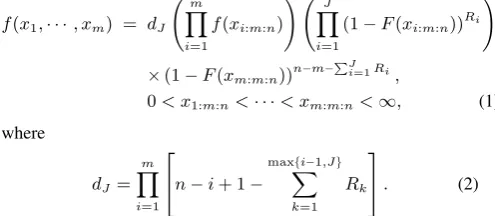
Supposenitems on a life-testing experiment and the experimenter provides a time T. If the failure times of the items are from a continuous population with cumulative distribution function (CDF) F(x)and probability density function (PDF)f(x). Then, the joint density function of the adaptive Type-II progressively censored sampleX = (X1,m,n, ..., Xm,m,n)with censoring schemeR = (R1, ..., Rm)is then given by (see Ng et al., 2009)

f(x1,· · ·, xm) = dJ m

Y

i=1

f(xi:m:n)

! J

Y

i=1

(1−F(xi:m:n))Ri

!

×(1−F(xm:m:n))n−m− PJ

i=1Ri_,

0< x1:m:n<· · ·< xm:m:n<∞, (1) where

dJ =

m

Y

i=1



n−i+ 1−

max{i−1,J}

X

k=1 Rk



. (2)

In this paper, the underlying distribution is assumed to be the two-parameter generalized exponential distribution which is introduced by Gupta and Kundu (1999) as an alternative to the gamma and Weibull distributions. The two-parameter generalized exponential distribution has PDF and CDF are given, respectively, by

f(x;α, β) = α

β e

−x

β₍₁₋_e−xβ₎α−1_{, x >}₀_, ₍₃₎

F(x;α, β) = (1−e−xβ₎α_{, x >}₀_, ₍₄₎

(3)

From (1), (3) and (4), we obtain the likelihood function ofαandβ, based on the adaptive Type-II progressively censored sampleX= (X1:m:n, ..., Xm:m:n)with censoring schemeR= (R1, ..., Rm), as

L(x;θ, σ) = dJ m

Y

i=1 θ

σe

−xi_σ

(1−e−xiσ₎θ−1

J

Y

i=1

(1−(1−e−xiσ₎θ₎Ri

×

1−1−e−xmσ

θn−m−

PJ i=1Ri

, (5)

wheredJis defined in (2).

3. THE POSTERIOR DISTRIBUTION

In this section, we derive the joint and conditional posterior distri-butions of the two unknown parametersθandσ. Under the assump-tion that both parametersθandσare unknown and independent, we may consider the prior distributions ofθandσas independent gamma prior distributions, G(a, b) and G(c, d), respectively:

π1(c) = baca−1e−bc

Γ(a) , c >0, (6)

and

π2(β) = ξγβγ−1e−ξβ

Γ(γ) , β >0 (7)

Multiplying π1(θ|a, b) by π2(σ|c, d), we obtain the joint prior function ofθandσas

π(θ, σ) = b

a_dc

Γ(a)Γ(c)θ

a−1_σc−1_exp(₋_bθ₋_dσ₎_. ₍₈₎

Using the likelihood function given in (5) and the joint prior given in (8), the joint posterior function ofθandσcan be obtained as

π∗(θ, σ|x) ∝ θm+a−1_σ−m+c−1_e−bθ−dσ

"m

Y

i=1 e−xiσ

1−e−xiσ

θ−1 # × "_J Y i=1

1−1−e−xiσ

θRi#

×1−(1−e−xmσ ₎θ

n−m−PJ i=1Ri

. (9)

From (9), the conditional posterior density function ofθ givenσ can be obtained as

π∗_θ(θ|σ,x) ∝ θm+a−1_e−bθ

"m

Y

i=1

(1−e−xiσ₎θ−1

# × "_J Y i=1

1−1−e−xiσ

θRi #

×

1−1−e−xmσ

θn−m−

PJ i=1Ri

. (10)

Similarly, the conditional posterior density function ofσgivenθ can be obtained as

πσ∗(σ|θ,x) ∝ σ

−m+c−1 e−dσ

"m

Y

i=1 e−xiσ

1−e−xiσ

θ−1 # × " _J Y i=1

1−1−e−xiσ

θRi#

×

1−1−e−xm_σ θ

n−m−PJ i=1Ri

. (11)

Unfortunately, the conditional posterior distribution ofθandσin (10) and (11) cannot be reduced analytically to well known distri-butions and therefore it is not possible to sample directly by stan-dard methods, but the plot of it show that it is similar to normal dis-tribution. So, to generate random numbers from these distributions, we use the M-H algorithm within the Gibbs Sampling scheme with normal proposal distribution.

4. TWO-SAMPLE BAYESIAN PREDICTION FOR FUTURE ORDER STATISTICS

One of the main objectives of statistical modeling is to pre-dict future observations on the basis of available information and Bayesian methodology provides a natural way. Several authors ad-dressed the issue of prediction and obtained the predictive bounds for future data. The aim of this section is to discuss the problem of predicting unobserved order statistics from the future sample from the generalized exponential distribution on the basis of an observed (informative) adaptive Type-II progressive censored data from the same distribution. The predictive density and distribution functions are obtained and used to determine prediction intervals for the un-observed order statistics. We consider the prediction problem in terms of the estimation of the posterior predictive density of a fu-ture observation for two-sample prediction case. We also construct predictive interval for the observed order statistics observation us-ing Gibbs samplus-ing procedure.

Suppose thatXR

1:m:n, X2:m:nR , ..., Xm:m:nR is the observed adaptive Type-II progressively censored sample drawn from the general-ized exponential distribution andY1:N, Y2:N, ..., YN:N are unob-served order statistics from an independent future random sample (of sizeN) from the same distribution. Based on the observed adap-tive Type-II progressively censored sample, our aim is to construct Bayesian prediction for thesth_{order statistics,}_Ys:N,₁_{< s < N.} The marginal density function ofYs:N, givenθ >0andσ >0, is of the form:

g(s)(ys|θ, σ) =D(s)f(ys|θ, σ) [F(ys|θ, σ)]s−1[1−F(ys|θ, σ)]n−s, (12) whereD(s) = n!

(n−s)!(s−1)!.

By substituting from(3)and(4)into (12), we obtain the marginal density and distribution functions ofYs:N, respectively, as

g(s)(ys|θ, σ) =D(s)θ

σe

−ys_σ

(1−e−ysσ₎θs−1

h

1−(1−e−ysσ₎θ

in−s

=D(s)θ

σe

−ys_σ

n−s

X

k=o

ak(s)(1−e−ysσ ₎θ(k+s)−1

(4)

and

G(s)(ys|θ, σ) =D(s)

n−s

X

k=o ak(s)

"

(1−e−ysσ₎θ(k+s)

k+s

#

, (14)

whereak(s) = (−1)k n−s k

.

The Bayesian predictive density function ofYs:N, based on the served adaptive Type-II progressively censored sample, can be ob-tained as

g∗_(s)(ys|θ, σ) =

Z ∞

0

Z ∞

0

g(s)(ys|θ, σ)Π∗(θ, σ|x)dθdσ, (15)

whereΠ∗₍_{θ, σ}_|_x₎_{is the joint posterior density of}_θ_and_σ_{as given}

in (9). Thus, the predictive distribution function, based on the ob-served adaptive Type-II progressively censored sample, is given by

G∗(s)(ys|θ, σ) =

Z ∞

0

Z ∞

0

G(s)(ys|θ, σ)Π∗(θ, σ|x)dθdσ. (16)

It is clear that g∗

(s)(ys|θ, σ) in (15), and G∗(s)(ys|θ, σ) in (16) cannot be expressed in closed form and hence it cannot be eval-uated analytically. A simulation based on consistent estimator g∗

(s)(ys|θ, σ), and G

∗

(s)(ys|θ, σ) can be obtained by using the MCMC-Gibbs sampling procedure with M-H, which is introduced by Metropolis et al. (1953) and then it is extended by Hastings (1970). We propose the following scheme to generate θ and σ from the posterior density functions and in turn obtain the simula-tion estimators of the predictive density and distribusimula-tion funcsimula-tions, g∗

(s)(ys|θ, σ)andG

∗

(s)(ys|θ, σ), forYs:N.

(1) Start with an (θ(0)_,_σ(0)_).

(2) Seti= 1.

(3) Generate θ(i) _from _π∗

θ(θ|σ,x) with the N(θ

(i−1)_{, V ar}_(ˆ_θ₎₎ proposal distribution.

(4) Generateσ(i) _from _π∗

σ(σ|θ,x) with theN(σ(i−1), V ar(ˆσ)) proposal distribution.

(5) Computeθ(i)_and_σ(i)_.

(6) Seti=i+ 1

(7) Repeat steps3−6 N1times.

(8) The simulation estimators of the predictive density and distri-bution functions,g∗

(s)(ys|θ, σ)andG

∗

(s)(ys|θ, σ), forYs:Ncan be obtained, respectively, as:

g∗_(s)(ys|θ, σ) = 1

N1−M1

N1

X

i=M1+1

g(s)(ys|θi, σi) (17)

and

G∗(s)(ys|θ, σ) =

1

N1−M1

N1

X

i=M1+1

G(s)(ys|θi, σi). (18)

whereM1is burn-in.

Moreover, a symmetric100(1−γ)%predictive interval forYs:N, s= 1,2, ..., N, can be obtained by solving the two following non-linear equations

P[Ys> L|x] = γ 2 = 1−

ˆ

G∗(s)(ys|θ, σ) =⇒Gˆ

∗

(s)(ys|θ, σ) = 1− γ

2,

(19)

and

P[Ys> U|x] = 1−γ

2 = 1−Gˆ ∗

(s)(ys|θ, σ) =⇒Gˆ

∗

(s)(ys|θ, σ) = γ

2,

(20) whereLandU are the lower and upper bounds of the predictive interval.

5. NUMERICAL RESULTS

5.1 Simulation study

A simulation study is carried out for evaluating the performance of the inferential methods discussed in the paper. We chosen= 30, m= 10andR= (3,2,3,1,2,3,1,0,2,3). ForT = 0.8, we first describe the algorithm, proposed by Ng et al. (2009), to generate adaptive Type-II progressively censored sample from the general-ized exponential distribution with parameters(θ, σ) = (2,3).

(1) Generate an ordinary Type-II progressively censored sample

X1,m,n, ..., Xm,m,n with the given censoring schemeR =

(R1, ..., Rm)from the GE distribution using the proposed al-gorithm in Balakrishnan and Sandhu (1995).

(2) Determine the value ofJ, whereXJ:m:n< T < XJ+1:m:n, and discard the sampleXJ+2,m,n, ..., Xm,m,n.

(3) Generate the firstm−J−1order statistics from a truncated distributionf(x)/[1−F(xj+1:m:n)]with sample size(n−

PJ

i=1Ri−J−1)asXj+2:m:n, Xj+3:m:n, ..., Xm:m:n, where f(x)andF(x)are given in (2.3) and (2.4), respectively.

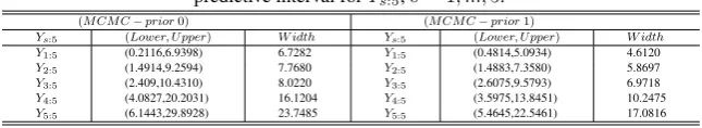
We used the above algorithm to generate adaptive Type-II pro-gressively censored sample and then computed the lower and up-per bounds of the100(1−γ)%predictive interval of the order statisticYs:N, s = 1,2, ..., N, from a future random sample of sizeN = 5 based on (N1 = 11000) MCMC samples and dis-card the first (M1 = 1000) values as burn-in. We replicated the process 1000 times and compute the average values of the lower bound, upper bound and width of the100(1−γ)%predictive inter-val whenγ = 0.01,0.05,0.10,0.20. The results are obtained us-ing the non-informative gamma priors for the two parameters with a=b=c=d= 0(we call it MCMC - prior 0) and the informa-tive gamma priors for the two parameters witha= 1,b= 2,c= 1

andd= 2(we call it MCMC - prior 1). The obtained results are presented in Tables 1-4.

From the results obtained in Tables 1-4, it can be observed that the Bayesian prediction intervals with informative priors are tighter than the width of those with noninformative priors. Also, when the significant level (γ) increases, the width of the prediction interval decreases in all cases. Moreover, the width of all prediction inter-vals increase with increasings.

5.2 Numerical example

To illustrate the inferential procedures developed in the preceding sections, we consider the following data giving the number of mil-lion revolutions before failure for each of 23 ball bearings in the life test. These data are taken from Lawless (1982, Page 228) and has been used earlier by Gupta and Kundu (2002)

17.88 28.92 33.00 41.52 42.12 45.60 48.80 51.84

51.96 54.12 55.56 67.80

68.64 68.64 68.88 84.12 93.12 98.64 105.12 105.84 127.92 128.04 173.40

(5)

T = 45and R=(2,0,1,3,0,0,2,0,1,4). Thus, the generated adaptive Type-II progressively censored sample is

42.12, 51.96, 54.12, 67.8, 68.64, 84.12, 93.12, 98.64, 105.12, 105.84, 127.92, 128.04, 173.4

Because we have no prior information about the unknown param-eters, we assume here the non-informative prior (witha = b =

c = d = 0). Based on the generated adaptive Type-II progres-sively censored sample, we compute the lower and upper bounds of the100(1−γ)%predictive interval of the order statisticYs:N, s= 1,2, ..., N, from a future random sample of sizeN = 5. The lower bound, upper bound and width of the99%and 95% pre-dictive intervals are presented in Table 5. The lower bound, upper bound and width of the90%and80%predictive intervals are pre-sented in Table 6.

5.3 Conclusion

In this paper, we discussed the problem if predicting unobserved order statistics from a future sample based on observed adaptive Type-II progressively censored sample from the generalized distri-bution. We derived the joint and conditional posterior functions for the unknown parameters. Also, we used the MCMC-Gibbs sam-pling procedure with M-H to estimate the predictive density and distribution functions ofYs:Nand then calculated the Bayesian pre-diction interval ofYs:N,s = 1, ....N. From all obtained results in the simulation study and the numerical example, we can notice that the Bayesian prediction interval with informative prior is better than that with noninformative prior.

6. REFERENCES

1. Amein, M.M. (2016). Estimation for Unknown Parameters of the Burr Type-XII Distribution Based on an Adaptive Progres-sive Type-II Censoring Scheme. Journal of Mathematics and Statistics12, 119-126.

2. Amein, M.M. (2017). Estimation for Unknown Parameters of the Extended Burr Type-XII Distribution Based on an Adaptive Type-II Progressive Censoring Scheme,Global Journal of Pure and Applied Mathematics13, 7709-7724.

3. Balakrishnan, N. (2007). Progressive censoring methodology: An appraisal (with discussions).Test16, 211-296.

4. Balakrishnan, N. and Aggarwala, R. (2000).Progressive Cen-soring: Theory, Methods, and Applications, Birkhauser, Boston, Berlin .

5. Bernardo, J.M. (1988). Bayesian linear probabilistic classifca-tion. In: Gupta, S.S., Berger, J.O. (Eds.), Statistical Decision Theory and Related Topics IV, vol. 1. Springer, Berlin, pp. 151162.

6. Brown, P.J. and Makalainen, T. (1992). Regression, sequen-tial measurements and coherent calibration. In: Bernardo, J.M., Berger, J.O., Dawid, A.P., Smith, A.F.M. (Eds.), Bayesian Statis-tics 4. Oxford University Press, Oxford, pp. 97108 (with discus-sion).

7. Cramer, E. and Iliopoulos, G. (2010). Adaptive progressive Type-II censoring.Test 9, 342-358.

8. Devroye, L. and Gyorfi, L. (1985).Nonparametric Density Es-timation: TheL1View, Wiley, New York.

9. Gupta, R.D. and Kundu, D. (1999). Generalized exponential dis-tribution. Australian & New Zealand Journal of Statistics 41

173-188.

10. Hastings, W.K. (1970). Monte Carlo sampling methods using Markovchains and their applications.Biometrika57, 97-109.

11. Lawless, J.F. (1982).Statistical models and methods for life-time data. New York: Wiley.

12. Mahmoud, M.A.W., Soliman, A.A., Abd Ellah, A.H., El-Sagheer, R.M. (2013). Estimation of Generalized Pareto under an Adaptive Type-II Progressive Censoring,”Intelligent Infor-mation Management5, 73 -83.

13. Metropolis, N., Rosenbluth, A. W., Rosenbluth, M. N., Teller, A. H. and Teller, E.(1953). Equations of State Calculations by fast Computing Machines,Journal Chemical Physics21, 1087-1091.

14. Mohie El-Din, M. M. M., Amein, M. M., Shafay, A. R. and Mohamed, S. (2017). Estimation of generalized exponential dis-tribution based on an adaptive progressively type-II censored sample,Journal of Statistical Computation and Simulation87, 1292-1304.

15. Mohie El-Din, M.M. and Shafay, A.R. (2013). One- and Two-Sample Bayesian Prediction Intervals Based on Progressively Type-II Censored Data.Statistical papers54, 287-307. 16. Nelson, W. (1982).Applied life data analysis. NewYork:

Wi-ley.

17. Ng, H.K.T and Chan, P.S. (2007). Discussion on Progressive censoring methodology: an appraisal by N. Balakrishnan.Test

16, 287-289.

(6)

Table 1. The average values of the lower bound, upper bound and width of the99%

predictive interval forYs:5,s= 1, ...,5.

(M CM C−prior0) (M CM C−prior1)

Ys:5 (Lower, U pper) W idth Ys:5 (Lower, U pper) W idth

Y1:5 (0.0399,10.4585) 10.4186 Y1:5 (0.1369,7.5849) 7.4480 Y2:5 (0.2819,11.8369) 11.5550 Y2:5 (0.6881,10.5882) 9.9001 Y3:5 (1.3206,18.6678) 17.3471 Y3:5 (1.3285,15.3512) 14.0227 Y4:5 (2.4704,44.7430) 42.2726 Y4:5 (2.2304,22.5209) 20.2905 Y5:5 (3.9501,47.4535) 43.5034 Y5:5 (3.6449,39.2798) 35.6349

Y1:5 (0.2787,7.7365) 7.4578 Y1:5 (0.2812,5.9442) 5.6630 Y2:5 (1.2391,9.5651) 8.3259 Y2:5 (1.1009,8.4139) 7.3130 Y3:5 (2.1861,13.6587) 11.4726 Y3:5 (2.077,11.9393) 9.8622 Y4:5 (3.5211,26.4485) 22.9274 Y4:5 (3.1976,17.2451) 14.0474 Y5:5 (4.7753,37.5113) 32.7359 Y5:5 (5.0236,32.3138) 27.2901

Y1:5 (0.2116,6.9398) 6.7282 Y1:5 (0.4814,5.0934) 4.6120

Y2:5 (1.4914,9.2594) 7.7680 Y2:5 (1.4883,7.3580) 5.8697 Y3:5 (2.409,10.4310) 8.0220 Y3:5 (2.6075,9.5793) 6.9718

[image:6.595.140.471.203.260.2]

Y4:5 (4.0827,20.2031) 16.1204 Y4:5 (3.5975,13.8451) 10.2475 Y5:5 (6.1443,29.8928) 23.7485 Y5:5 (5.4645,22.5461) 17.0816

Y1:5 (0.5926,5.0386) 4.4460 Y1:5 (0.8192,4.2796) 3.4604

Y2:5 (1.8149,8.5751) 6.7602 Y2:5 (1.8038,6.3711) 4.5673 Y3:5 (3.119,10.2792) 7.1601 Y3:5 (2.9292,8.8177) 5.8885

Y4:5 (4.6125,13.3709) 8.7584 Y4:5 (4.3643,12.0921) 7.7277 Y5:5 (6.7396,20.8389) 14.0993 Y5:5 (6.4141,19.7169) 13.3027

Table 5. The average values of the lower bound, upper bound and width of the99%and95%

predictive interval forYs:5,s= 1, ...,5. 99%predictive intervals 95%predictive intervals

Y1:5 (5.3360,88.9052) 83.5692 Y1:5 (10.7497,72.2713) 61.5216 Y2:5 (19.2642,109.4150) 90.1511 Y2:5 (21.5242,100.3500) 78.8256 Y3:5 (24.9427,153.6400) 128.6970 Y3:5 (32.8750,126.6540) 93.7792 Y4:5 (36.2476,226.0080) 189.7600 Y4:5 (44.9061,164.7790) 119.873 Y5:5 (49.3578,336.7620) 287.4040 Y5:5 (63.9343,337.0110) 273.077

Table 6. The average values of the lower bound, upper bound and width of the90%and80%

predictive interval forYs:5,s= 1, ...,5. 90%predictive intervals 80%predictive intervals

[image:6.595.144.467.307.366.2]