First Order vs Higher Order Modification in Distributional Semantics

First-order vs. higher-order modification in distributional semantics

Gemma Boleda Linguistics Department University of Texas at Austin [email protected]

Eva Maria Vecchi Center for Mind/Brain Sciences

University of Trento

[email protected]

Miquel Cornudella and Louise McNally Departament de Traducci´o i Ci`encies del Llenguatge

Universitat Pompeu Fabra

[email protected],[email protected]

Abstract

Adjectival modification, particularly by ex-pressions that have been treated as higher-order modifiers in the formal semantics tradi-tion, raises interesting challenges for semantic composition in distributional semantic els. We contrast three types of adjectival mod-ifiers – intersectively used color terms (as in

whitetowel, clearly first-order), subsectively used color terms (whitewine, which have been modeled as both first- and higher-order), and intensional adjectives (formerbassist, clearly higher-order) – and test the ability of different composition strategies to model their behav-ior. In addition to opening up a new empir-ical domain for research on distributional se-mantics, our observations concerning the at-tested vectors for the different types of adjec-tives, the nouns they modify, and the resulting noun phrases yield insights into modification that have been little evident in the formal se-mantics literature to date.

1 Introduction

One of the most appealing aspects of so-called dis-tributional semantic models (see Turney and Pan-tel (2010) for a recent overview) is that they af-ford some hope for a non-trivial, computationally tractable treatment of the context dependence of lex-ical meaning that might also approximate in inter-esting ways the psychological representation of that meaning (Andrews et al., 2009). However, in or-der to have a complete theory of natural language meaning, these models must be supplied with or connected to a compositional semantics; otherwise,

we will have no account of the recursive potential that natural language affords for the construction of novel complex contents.

In the last 4-5 years, researchers have begun to introduce compositional operations on distribu-tional semantic representations, for instance to com-bine verbs with their arguments or adjectives with nouns (Erk and Pad´o, 2008; Mitchell and Lapata, 2010; Baroni and Zamparelli, 2010; Grefenstette and Sadrzadeh, 2011; Socher et al., 2011)1. Al-though the proposed operations have shown vary-ing degrees of success in a number of tasks such as detecting phrase similarity and paraphrasing, it re-mains unclear to what extent they can account for the full range of meaning composition phenomena found in natural language. Higher-order modifica-tion (that is, modificamodifica-tion that cannot obviously be modeled as property intersection, in contrast to first-order modification, which can) presents one such challenge, as we will detail in the next section.

The goal of this paper is twofold. First, we exam-ine how the properties of different types of adjecti-val modifiers, both in isolation and in combination with nouns, are represented in distributional mod-els. We take as a case study three groups of adjec-tives: 1) color terms used to ascribe true color prop-erties (referred to here asintersectivecolor terms), as prototypical representative of first-order modi-fiers; 2) color terms used to ascribe properties other than simple color (here,subsectivecolor terms), as representatives of expressions that could in principle

1

In a complementary direction, Garrette et al. (2011) con-nect distributional representations of lexical semantics to logic-based compositional semantics.

be given a well-motivated first-order or higher-order analysis; and 3)intensionaladjectives (e.g.former), as representative of modifiers that arguably require a higher-order analysis. Formal semantic models tend to group the second and third groups together, de-spite the existence of some natural language data that questions this grouping. However, our results show that all three types of modifiers behave differ-ently from each other, suggesting that their semantic treatment needs to be differentiated.

Second, we test how five different composition functions that have been proposed in recent literature fare in predicting the attested properties of nominals modified by each type of adjective. The model by Baroni and Zamparelli (2010) emerges as a suitable model of adjectival composition, while multiplica-tion and addimultiplica-tion shed mixed results.

The paper is structured as follows. Section 2 pro-vides the necessary background on the semantics of adjectival modification. Section 3 presents the meth-ods used in our study. Section 4 describes the char-acteristics of the different types of adjectival modifi-cation, and Section 5, the results of the composition operations. The paper concludes with a general dis-cussion of the results and prospects for future work.

2 The semantics of adjectival modification

Accounting for inference in language is an impor-tant concern of semantic theory. Perhaps for this rea-son, within the formal semantics tradition the most influential classification of adjectives is based on the inferences they license (see (Parsons, 1970) and (Kamp, 1975) for early discussion). We very briefly review this classification here.

First, so called intersective adjectives, such as (the literally used)white inwhite dress, yield the infer-ence that both the property contributed by the ad-jective and that contributed by the noun hold of the individual described; in other words, a white dress is white and is a dress. The semantics for such mod-ifiers is easily characterized in terms of the intersec-tion of two first-order properties, that is, properties that can be ascribed to individuals.

On the other extreme, intensional adjectives, such

asformeroralleged informer/alleged criminal, do

not license the inference that either of the properties holds of the individual to which the modified

nom-inal is ascribed. Indeed, such adjectives cannot be used as predicates at all:

(1) ??The criminal was former/alleged.

The infelicity of (1) is generally attributed to the fact that these adjectives do not describe individu-als directly but rather effect more complex opera-tions on the meaning of the modified noun. It is for this reason that these adjectives can be considered higher-order modifiers: they behave as properties of properties. Though rather abstract, the higher-order analysis is straightforwardly implementable in for-mal semantic models and captures a range of lin-guistic facts successfully.

Finally, subsective adjectives such as (the non-literally-used)white inwhite wine, consitute an in-termediate case: they license the inference that the property denoted by the noun holds of the indi-vidual being described, but not the property con-tributed by the adjective. That is, white wine is not white but rather a color that we would proba-bly call some shade of yellow. This use of color terms, in general, is distinguished primarily by the fact that color serves as a proxy for another prop-erty that is related to color (e.g. type of grape), though the color in question may or may not match the color identified by the adjective on the intersec-tive use (see (G¨ardenfors, 2000) and (Kennedy and McNally, 2010) for discussion and analysis). The effect of the adjective, rather than to identify a value for an incidentalCOLORattribute of an object, is of-ten to characterize a subclass of the class described by the noun (white wine is a kind of wine, brown rice a kind of rice, etc.).

pred-icative adjectives such as happy than they do with adjectives such asformer.

The trio of intersective color terms, subsective color terms, and intensional adjectives provides fer-tile ground for exploring the different composition functions that have been proposed for distributional semantic representations. Most of these functions start from the assumption that composition takes pairs of vectors (e.g. a verb vector and a noun vec-tor) and returns another vector (e.g. a vector for the verb with the noun as its complement), usually by some version of vector addition or multiplication (Erk and Pad´o, 2008; Mitchell and Lapata, 2010; Grefenstette and Sadrzadeh, 2011). Such func-tions, insofar as they yield representations which strengthen distributional features shared by the com-ponent vectors, would be expected to model inter-sective modification.

Consider the example of white dress. We might expect the vector fordressto include non-zero fre-quencies for words such as wedding and funeral. The vector for white, on the other hand, is likely to have higher frequencies forwedding than for

fu-neral, at least in corpora obtained from the U.S. and

the U.K. Combining the two vectors with an addi-tive or multiplicaaddi-tive operation should rightly yield a vector forwhite dresswhich assigns a higher fre-quency toweddingthan tofuneral.

Additive and multiplicative functions might also be expected to handle subsective modification with some success because these operations provide a natural account for how polysemy is resolved in meaning composition. Thus, the vector that results from adding or multiplying the vector forwhitewith that fordressshould differ in crucial features from the one that results from combining the same vector

forwhite with that forwine. For example,

depend-ing on the details of the algorithm used, we should find the frequencies of words such assnowormilky

weakened and words likestraworyellow strength-ened in combination withwine, insofar as the former words are less likely than the latter to occur in con-texts wherewhitedescribes wine than in those where it describes dresses. In contrast, it is not immedi-ately obvious how these operations would fare with intensional adjectives such asformer. In particular, it is not clear what specific distributional features of the adjective would capture the effect that the

ad-jective has on the meaning of the resulting modified nominal.

Interestingly, recent approaches to the semantic composition of adjectives with nouns such as Baroni and Zamparelli (2010) and Guevara (2010) draw on the classical analysis of adjectives within the Mon-tagovian tradition of formal semantic theory (Mon-tague, 1974), on which they are treated as higher or-der predicates, and model adjectives as matrices of weights that are applied to noun vectors. On such models, the distributional properties of observed oc-currences of adjective-noun pairs are used to induce the effect of adjectives on nouns. Insofar as it is grounded in the intuition that adjective meanings should be modeled as mappings from noun mean-ings to adjective-noun meanmean-ings, the matrix anal-ysis might be expected to perform better than ad-ditive or multiplicative models for adjective-noun combinations when there is evidence that the adjec-tive denotes only a higher-order property. There is also no a priori reason to think that it would fare more poorly at modeling the intersective and subsec-tive adjecsubsec-tives than would addisubsec-tive or multiplicasubsec-tive analyses, given its generality.

In this paper, we present the first studies that we know of that explore these expectations.

3 Method

We built a semantic space and tested the composi-tion funccomposi-tions as specified in what follows.

3.1 Semantic space

The semantic space we used for our experiments consists of a matrix where each row vector repre-sents an adjective, noun or adjective-noun phrase (henceforth, AN). We first introduce the source cor-pus, then the vocabulary that we represent in the space, and finally the procedure to build the vectors representing the vocabulary items from corpus data.

3.1.1 Source corpus

Our source corpus is the concatenation of the ukWaC corpus2, a mid-2009 dump of the English Wikipedia3 and the British National Corpus4. The corpus is tokenized, POS-tagged and lemmatized

2

http://wacky.sslmit.unibo.it/ 3

with TreeTagger (Schmid, 1995) and contains about 2.8 billion tokens. We extracted all statistics at the lemma level, ignoring inflectional information.

3.1.2 Vocabulary

The core vocabulary of the semantic space con-sists of the 8K most frequent nouns and the 4K most frequent adjectives from the corpus. By crossing the set of 700 most frequent adjectives (reduced to 663 after removing questionable items like above, less

andvery) and the 4K most frequent nouns and se-lecting those ANs that occured at least 100 times in the corpus, we obtained a set of 179K ANs that we added to the semantic space, for a total of 191K rows. These ANs were used for training the linear models as well as for providing a basis for the anal-ysis of the results.

3.1.3 Semantic space parameters

The dimensions (columns) of our semantic space are the top 10K most frequent content words in the corpus (nouns, adjectives, verbs and adverbs), ex-cluding the 300 most frequent words ofallparts of speech.

For each word or AN, we collected raw co-occurrence counts by recording their sentence-internal co-occurrence with each of words in the di-mensions. The counts were then transformed into Local Mutual Information (LMI) scores, an associ-ation measure that closely approximates the com-monly used Log-Likelihood Ratio but is simpler to compute (Evert, 2005). Specifically, given a row el-ementr, a column elementcand a counting function

C(r, c), then

LM I =C(r, c)·logC(r, c)C(∗,∗)

C(r,∗)C(∗, c) (1)

where C(r, c) is how many times r cooccurs with

c, C(r,∗) is the total count ofr, C(∗, c) is the to-tal count of c, and C(∗,∗) is the cumulative co-occurrence count of anyrwith anyc.

The dimensionality of the space was reduced us-ing Sus-ingular Value Decomposition (SVD), as in La-tent Semantic Analysis and related distributional semantic methods (Landauer and Dumais, 1997; Rapp, 2003; Sch¨utze, 1997). Both LMI and SVD were used for the core vocabulary, and the AN vec-tors were computed based on the values for the

core vocabulary. All of the results discussed in the article are based on the SVD-reduced space, be-cause it yielded consistently better results, except for those involving multiplicative composition, which was carried out on the non-reduced model because SVD reduction introduces negative values for the la-tent dimensions used for the reduced space.

Some of the parameters of the space and com-position functions were set based on performance on independent word similarity and AN similarity tasks (Rubenstein and Goodenough, 1965; Mitchell and Lapata, 2010). In addition to LMI, we tested the performance using log-transformed frequencies and found very poor performance in the aforemen-tioned tasks. The number of latent dimensions for the SVD-reduced space was set at 300 after testing the performance using 300, 600 and 900 latent di-mensions.

In the discussion, we use the cosine of two vectors as a measure of similarity. This is the most common choice in related work, as it has shown to be robust across different tasks and settings, though other op-tions (in particular, measures that are not symmetric or do not normalize) could be explored (Widdows, 2004).

3.2 Composition models

The experiments described below were carried out using five compositional methods that have been ex-plored in recent studies of compositionality in dis-tributional semantic spaces (Mitchell and Lapata, 2010; Guevara, 2010; Baroni and Zamparelli, 2010). For each function, we definep as the composition of the adjective vector, u, and the noun vector, v, a nomenclature that follows Mitchell and Lapata (2010).

Additive (add) AN vectors were obtained by summing the corresponding adjective and noun vec-tors. We also explored the effects of the additive model with normalized component adjective and noun vectors (addn).

p=u+v (2)

Multiplicative(mult) AN vectors were obtained by component-wise multiplication of the adjective and noun vectors in the non-reduced semantic space.

Dilation(dl) AN vectors were obtained by calcu-lating the dot products ofu·uandu·vand stretching

vby a factorλ(in our case, 16.7) in the direction of

u (Clark et al., 2008; Mitchell and Lapata, 2010). The effect of this operation is to “stretch” the head vectorv (noun, in our case) in the direction of the modifying vectoru(adjective).

p= (u·u)v+ (λ−1)(u·v) (4)

The factorλwas selected based on the optimal pa-rameters presented in Mitchell and Lapata (2010). We tested both reported values (16.7 and 2.2) and foundλ= 16.7to perform better in terms of rank of observed equivalent (see Section 5).

The preceding functions produce an AN vector from the component A and N vectors. The remain-ing two functions do not use the vector for the ad-jective, but learn a matrix representation for it. The composed AN vector is obtained by multiplying the matrix by the noun vector. The general equation for the two functions is the following, whereBis a ma-trix of weights that is multiplied by the noun vector

vto produce the AN vectorp.

p=Bv (5)

In the linear map (lim) approach proposed by Guevara (2010), one single matrix B is learnt that represents all adjectives. An AN vector is obtained by multiplying the weight matrix by the concate-nation of the adjective and noun vectors, so that each dimension of the generated AN vector is a lin-ear combination of dimensions of the correspond-ing adjective and noun vectors. In our implementa-tion,Bis an 300 x 300 weight matrix representing an adjective, and v is a 300-dimension noun vec-tor. Following Guevara (2010), we estimate the co-efficients of the equation using (multivariate) partial least squares regression (PLSR) as implemented in the Rplspackage (Mevik and Wehrens, 2007), set-ting the latent dimension parameter of PLSR to 300. This value was chosen after testing values 100, 200 and 300 on the AN similarity tasks (Mitchell and Lapata, 2010). Coefficient matrix estimation is per-formed by feeding PLSR a set of input-output exam-ples, where the input is given by concatenated ad-jective and noun vectors, and the output is the vector of the corresponding AN directly extracted from our

semantic space. The matrix is estimated using a ran-dom sample of 2.5K adjective-noun-AN tuples.5

In theadjective-specific linear map(alm) model, proposed by Baroni and Zamparelli (2010), a dif-ferent matrix B is learnt for each adjective. The weights of each of the rows of the weight matrix are the coefficients of a linear equation predicting the values of one of the dimensions of the normal-ized AN vector as a linear combination of the di-mensions of the normalized component noun. The linear equation coefficients are estimated again us-ing PLSR, and in the present implementation we use ridge regression generalized cross-validation (GCV) to automatically choose the optimal ridge parameter for each adjective (Golub et al., 1979). This pro-cedure drastically outperforms setting a fixed num-ber of dimensions. The model is trained on all N-AN vector pairs available in the semantic space for each adjective, and range from 100 to over 1K items across the adjectives we tested.

3.3 Datasets

We built two datasets of adjective-noun phrases for the present research, one with color terms and one with intensional adjectives.6

Color terms. This dataset is populated with a ran-domly selected set of adjective-noun pairs from the space presented above. From the 11 colors in the ba-sic set proposed by Berlin and Kay (1969), we cover

7 (black, blue, brown, green, red, white, and

yel-low), since the remaining (grey, orange, pink, and

purple) are not in the 700 most frequent set of

ad-jectives in the corpora used. From an original set of 412 ANs, 43 were manually removed because of suspected parsing errors (e.g.white photograph, for

black and white photograph) or because the head

noun was semantically transparent (white variety). The remaining 369 ANs were tagged independently by the second and fourth authors of this paper, both native English speaker linguists, asintersective(e.g.

white towel), subsective (e.g. white wine), or

id-iomatic, i.e. compositionally non-transparent (e.g.

black hole). They were allowed the assignment of at

5

most two labels in case of polysemy, for instance for

black staff for the person vs. physical object senses

of the noun oryellow skinfor the race vs. literally painted interpretations of the AN. In this paper, only the first label (most frequent interpretation, accord-ing to the judges) has been used. Theκcoefficient of the annotation on the three categories (first interpre-tation only) was 0.87 (conf. int. 0.82-0.92, according to Fleiss et al. (1969)), observed agreement 0.96.7 There were too few instances of idioms (17) for a quantitative analysis of the sort presented here, so these are collapsed with the subsective class in what follows.8 The dataset as used here consists of 239 intersective and 130 subsective ANs.

Intensional adjectives. The intensional dataset contains all ANs in the semantic space with a pre-selected list of 10 intensional adjectives, manually pruned by one of the authors of the paper to elimi-nate erroneous examples and to ensure that the ad-jective was being intensionally used. Examples of the ANs eliminated on these grounds include past

twelve (cp. accepted past president), former girl

(probablyformer girl friendor similar),false rumor

(which is a real rumor that is false, vs. e.g. false

floor, which is not a real floor), ortheoretical work

(which is real work related to a theory, vs. e.g.

theo-retical speed, which is a speed that should have been

reached in theory). Other AN pairs were excluded on the grounds that the noun was excessively vague (e.g. past one) or because the AN formed a fixed expression (e.g. former USSR). The final dataset contained 1,200 ANs, distributed as follows:former

(300 examples),possible(244),future(243), poten-tial(183),past(87), false(44),apparent (39),

arti-ficial(36),likely(18),theoretical(6).9

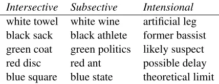
Table 1 contains examples of each type of AN we are considering.

7_{Code for the computation of inter-annotator agreement by} Stefan Evert, available at http://www.collocations. de/temp/kappa_example.zip.

8

An alternative would have been to exclude idiomatic ANs from the analysis.

9_{Alleged, one of the most prototypical intensional adjectives,} is not considered here because it was not among the 700 most frequent adjectives in the space. We will consider it in future work.

Intersective Subsective Intensional

white towel white wine artificial leg black sack black athlete former bassist green coat green politics likely suspect red disc red ant possible delay blue square blue state theoretical limit

Table 1: Example ANs in the datasets.

4 Observed vectors

We began by exploring the empirically observed vectors for the adjectives (A), nouns (N), and adjective-noun phrases (AN) in the datasets, as they are represented in the semantic space. Note that we are working with the AN vectors directly har-vested from the corpora (that is, based on the co-occurrence of, say, the phrasewhite towelwith each of the 10K words in the space dimensions), with-out doing any composition. AN vectors obtained by composition will be examined in the following sec-tion. Though observed AN vectors should not be regarded as a gold standard in the sense of, for in-stance, Machine Learning approaches, because they are typically sparse10 and thus the vectors of their component adjective and noun will be richer, they are still useful for exploration and as a compari-son point for the composition operations (Baroni and Lenci, 2010; Guevara, 2010).

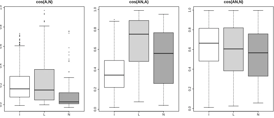
Figure 1 shows the distribution of the cosines be-tween A, N, and AN vectors with intensional adjec-tives (I, white box), intersective uses of color terms (IE, lighter gray box), and subsective uses of color terms (S, darker gray box).

In general, the similarity of the A and N vectors is quite low (cosine<0.2, left graph of Figure 1), and much lower than the similarities between both the AN and A vectors and the AN and N vectors. This is not surprising, given that adjectives and nouns de-scribe rather different sorts of things.

We find significant differences between the three types of adjectives in the similarity between AN and A vectors (middle graph of Figure 1). The adjec-tive and adjecadjec-tive-noun phrase vectors are nearer for

10

● ● ● ● ● ● ● ● ● ● ● ● ● ● ● ● ●

● ●

● ● ● ● ● ●

● ●

● ● ● ● ● ●

● ●

●

I L N

0.0

0.2

0.4

0.6

0.8

1.0

cos(A,N)

●

I L N

0.0

0.2

0.4

0.6

0.8

1.0

cos(AN,A)

I L N

0.0

0.2

0.4

0.6

0.8

1.0

cos(AN,N)

Figure 1: Cosine distance distribution in the different types of AN. We report the cosines between the component adjective and noun vectors (cos(A,N)), between the observed AN and adjective vectors (cos(AN,A)), and between the observed AN and noun vectors (cos(AN,N)). Each chart contains three boxplots with the distribution of the cosine scores (y-axis) for the intensional (I), intersective (IE), and subsective (S) types of ANs. The boxplots represent the value distribution of the cosine between two vectors. The horizontal lines in the rectangles represent the first quartile, median, and third quartile. Larger rectangles correspond to a more spread distribution, and their (a)symmetry mirrors the (a)symmetry of the distribution. The lines above and below the rectangle stretch to the minimum and maximum values, at most 1.5 times the length of the rectangle. Values outside this range (outliers) are represented as points.

intersective uses than for subsective uses of color terms, a pattern that parallels the difference in the distance between component A and N vectors. Since intersective uses correspond to the prototypical use of color terms (awhite dressis the color white, while

white wineis not), the greater similarity for the

in-tersective cases is unsurprising – it suggests that in the case of subsective adjectival modifiers, the noun “pulls” the AN further away from the adjective than happens with the cases of intersective modification. This is compatible with the intuition (manifest in the formal semantics tradition in the treatment of sub-sective adjectives as higher-order rather than first-order, intersective modifiers) that the adjective’s ef-fect on the AN in cases of subsective modification depends heavily on the interpretation of the noun with which the adjective combines, whereas that is less the case when the adjective is used intersec-tively.

As for intensional adjectives, the middle graph shows that their AN vectors are quite distant from the corresponding A vectors, in sharp contrast to what we find with both intersective and subsective

color terms. We hypothesize that the results for the intensional adjectives are due to the fact that they cannot plausibly be modeled as first order attributes (i.e. being potential or apparent is not a property in the same sense that beingwhiteoryellowis) and thus typically do not restrict the nominal description

per se, but rather provide information about whether

or when the nominal description applies. The re-sult is that intensional adjectives should be even weaker than subsectively used adjectives, in com-parison with the nouns with which they combine, in their ability to “pull” the AN vector in their direc-tion. Note, incidentally, that an alternative expla-nation, namely that the effect mentioned could be due to the fact that most nouns in the intensional dataset are abstract and that adjectives modifying abstract nouns might tend to be further away from their nouns altogether, is ruled out by the compari-son between the A and N vectors: the A-N cosines of the intensional and intersective ANs are similar. We thus conclude that here we see an effect of the

type of modificationinvolved.

the nearest neighbors of the intensional and of the color adjectives in the distributional space supports our hypothesized account of their contrasting be-haviors. We predict that the nearest neighbors are more dispersed for adjectives that cannot be mod-eled as first-order properties (i.e., intensional adjec-tives), than for those that can (here, the color terms). We find that the average cosine distance among the nearest ten neighbors of the intensional adjectives is 0.74 with a standard deviation of 0.13, which is sig-nificantly lower (t-test, p<0.001) than the average similarity among the nearest neighbors of the color adjectives, 0.96 with astandard deviation of 0.04.

Finally, with respect to the distances between the adjective-noun and head noun vectors (right graph of Figure 1), there is no significant difference for the intersective vs. subsective color terms. This can be explained by the fact that both kinds of modifiers are subsective, that is, the fact that a white dress is a dress and that white wine is wine.

In contrast, intensional ANs are closer to their component Ns than are color ANs (the difference is qualitatively quite small, but significant even for the intersective vs. intensional ANs according to a

t-test, p-value = 0.015). This effect, the inverse of what we find with the AN-A vectors, can similarly be explained by the fact that intensional adjectives do not restrict the descriptive content of the noun they modify, in contrast to both the intersective and subsective color ANs. Restriction of the nominal description may lead to significantly restricted dis-tributions (e.g. the phrase red button may appear in distinctively different contexts than doesbutton; similarly for green politicsand politics), while we do not expect the contexts in which former bassist

andbassistappear to diverge in a qualitatively

dif-ferent way because the basic nominal descriptions are identical, though further research will be neces-sary to confirm these explanations.

Finally, note that, contrary to predictions from some approaches in formal semantics, subsective color ANs and intensional ANs do not pattern to-gether: subsective ANs are closer to their nent As, and intensional ANs closer to their compo-nent Ns. This unexpected behavior underscores the fact highlighted in the previous paragraph: that the distributional properties of modified expressions are more sensitive to whether the modification restricts

the nominal description than to whether the modifier is intersective in the strictest sense of term.

We now discuss the extent to which the different composition functions account for these patterns.

5 Composed vectors

Since intersective modification is the point of com-parison for both subsective and intensional modifi-cation, we first discuss the composed vectors for the intersective vs. subsective uses of color terms, and then turn to intersective vs. intensional modification.

5.1 Intersective and subsective modification with color terms

To adequately model the differences between inter-sective and subinter-sective modification observed in the previous section, a successful composition function should yield a significantly smaller distance between the adjective and AN vectors for intersectively used adjectives, whereas it should yield no significant dif-ference for the distances between the noun and AN vectors.

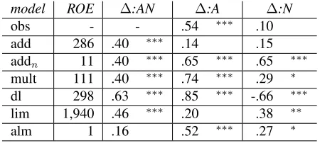
Table 2 provides a summary of the results with the observed data (obs) and the composition func-tions discussed in Section 3.2. The median rank of observed equivalent (ROE) is provided as a general measure of the quality of the composition function. It is computed by finding the cosine between the composed AN vectors and all rows in the semantic space and then determining the rank in which the ob-served ANs are found.11The remaining columns re-port the differences in standardized (z-score) cosines between the vector built with each of the composi-tion funccomposi-tions and the observed AN, A, and N vec-tors. A positive value means that the cosines for intersective uses are higher, while a negative value means that the cosines for subsective uses are higher. The first row (obs) contains a numerical summary of the tendencies for observed ANs explained in the previous section. This is the behavior that we expect to model.

Two composition functions come close to mod-eling the observed behavior: almandmult, though

almis better in terms of ROE, consistent with the

model ROE ∆:AN ∆:A ∆:N

obs - - .54 ∗∗∗ .10

add 286 .40 ∗∗∗ .14 .15 addn 11 .40 ∗∗∗ .65 ∗∗∗ .65 ∗∗∗

mult 111 .40 ∗∗∗ .74 ∗∗∗ .29 ∗ dl 298 .63 ∗∗∗ .85 ∗∗∗ -.66 ∗∗∗ lim 1,940 .46 ∗∗∗ .20 .38 ∗∗

alm 1 .16 .52 ∗∗∗ .27 ∗

Table 2: Intersective vs. subsective uses of color terms. The first column reports the rank of the observed equiva-lent (ROE), the rest report the differences (∆) betwen the intersective and subsective uses of color terms when com-paring the composed AN with the observed vectors for: AN, adjective (A), noun (N). See text for details. Signifi-cances according to a t-test: *** for p<0.001, **<0.01, *<0.05.

results reported in Baroni and Zamparelli (2010). In both cases, we find that these functions yield higher similarities for AN-A for the intersective than for the subsective uses of color terms, and a very slight (though still mildly significant) difference for the distance to the head noun. The addn function

performs very good in terms of ROE (median 11). This suggests that, for adjectival modification, pro-viding a vector that is in the middle of the two component vectors (which is what normalized ad-dition does) is a reasonable approximation of the observed vectors. However, precisely because the resulting vector is in the middle of the two com-ponent vectors, this function cannot account for the asymmetries in the distances found in the observed data. The non-normalized version also cannot ac-count for these effects because the adjective vec-tor, being much longer (as color terms are very fre-quent), totally dominates the AN, which results in no difference across uses when comparing to the ad-jective or to the noun.

The dilation model shows a strange pattern, as it yields a strongly significant negative difference in the AN-N distance. Thelimfunction exhibits the op-posite pattern as predicted, yielding no difference for the A similarities and a difference for the N similarities. A possible explanation for the AN- AN-A results is thatlimlearns from such a broad range of AN pairs that the impact of the distance between intersective vs. subsective uses of color terms from their component adjectives is dampened. Moreover,

limis by far the worst function in terms of ROE. All composition functions except foralmfind in-tersective uses easier to model. This is shown in the positive values in column∆:AN, which mean that the similarity between observed and composed AN vectors is greater for intersective than for subsective ANs. This is consistent with expectations. The sub-sective uses are specific to the nouns with which the color terms combine, and the exact interpretation of the adjective varies across those nouns. In contrast, the interpretation associated with intersective use is consistent across a larger variety of nouns, and in that sense should be predominantly reflected in the adjective’s vector. The exception in this respect is thealmfunction, since the weights for each adjec-tive matrix are estimated in relation to the noun vec-tors with which the adjective combines, on the one hand, and the related observed AN vectors, on the other; thus, the basic lexical representation of the adjective is inherently reflective of the distributions of the ANs in which it appears in a way that is not the case for the adjective representations used in the other composition models. And indeed,alm is the only function that shows no difference in difficulty (distance) between the predicted and observed AN vectors for intersective vs. subsective ANs.

Both mult and alm seem to account for the ob-served patterns in color terms. However, an exam-ination of the nearest neighbors of the composed ANs suggest thatalmcaptures the semantics of ad-jective composition in this case to a larger extent thanmult. For instance, the NN forblue square (in-tersective) are the following according tomul:blue,

red, official colour, traditional colour, blue

num-ber, yellow; while alm yields the following: blue

square, red square, blue circle, blue triangle, blue

pattern, yellow circle. Similarly, for green

poli-tics (subsective) mul yields: pleasant land, green

business,green politics,green issue,green strategy,

green product, whilealmyieldsgreen politics,green

movement, political agenda, environmental

move-ment,progressive government,political initiative.

5.2 Intensional modification

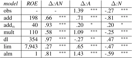
model ROE ∆:AN ∆:A ∆:N

obs - - 1.39 ∗∗∗ -.27 ∗∗∗

add 198 .66 ∗∗∗ .71 ∗∗∗ -.81 ∗∗∗ addn 40 .93 ∗∗∗ .20 ∗ .20 ∗

mult 110 .58 ∗∗∗ 1.09 ∗∗∗ -.25 ∗∗∗ dl 354 .97 ∗∗∗ -.27 ∗∗ .47 ∗∗∗ lim 7,943 .27 ∗∗∗ .65 ∗∗∗ -.47 ∗∗∗ alm 1 .81 ∗∗∗ 1.43 ∗∗∗ -.59 ∗∗∗

Table 3: Intersective vs. intensional ANs. Information as in Table 2.

them further (note the very poor performance oflim, though). As noted above, we expect more difficulty in modeling intensional modification vs. other kinds of modification, and this is verified in the results (cf. the positive values in second column). The dif-ference with the results in the previous subsection is that in this case the almfunction does present a higher difficulty in modeling intensional ANs, un-like with the color terms. This points to a qualitative difference between subsective and intensional adjec-tives that could be evidence for a first-order analysis of subsective color terms.

A good composition function should provide a large positive difference when comparing the AN to the A, and a small negative difference (because the effect is very small in the observed data) when comparing the AN to the N. The functions that best match the observed data are again alm and mult.

Add and lim show the predicted pattern, but to a much lesser degree (cf. smaller differences in col-umn ∆:A). Dl yields the exact opposite effect and

addn, though good in terms of ROE, is subject to

the problems discussed in the previous section. Again,almseems to be capturing relevant seman-tic aspects of composition with intensional adjec-tives. For instance, the nearest neighbors ofartificial legaccording toalmareartificial leg,artificial limb,

artificial joint,artificial hip,scar,small wound.

6 Discussion and conclusions

The present research provides some evidence for treating adjectives as matrices or functions, rather than vectors, although simple operations on vectors such as addition (for its excellent approximation to observed vectors) and multiplication (for its ability to reproduce the observed trends in the data) still

ac-count for some aspects of adjectival modification. The dilation model, in contrast, is not suitable for adjectival modification.

Our results also show that alm performs better than lim, but it is worth observing that it does so at the expense of modeling each adjective as a com-pletely different function. We considerlimvery at-tractive in principle because it generalizes across ad-jectives and is thus more parsimonious. Part of the poor results on lim were due to limitations of our implementation, as we trained the matrices on only 2.5K ANs, while our semantic space contains more than 170K ANs. However, the linguistic literature and the present results suggest that it might be use-ful to try a compromise betweenalmandlim, train-ing one matrix for each subclass of adjectives under analysis.

Beyond the new data it offers regarding the com-parative ability of the different composition func-tions to account for different kinds of adjectival modification, the study presented here underscores the complexity of modification as a semantic phe-nomenon. The role of adjectival modifiers as restric-tors of descriptive content is reflected differently in distributional data than is their role in providing in-formation about whether or when a description ap-plies to some individual. Formal semantic models, thanks to their abstractness, are able to handle these two roles with little difficulty, but also with limited insight. Distributional models, in contrast, offer the promise of greater insight into each of these roles, but face serious challenges in handling both of them in a unified manner.

Acknowledgments

References

Mark Andrews, Gabriella Vigliocco, and David Vinson. 2009. Integrating experiential and distributional data to learn semantic represenations. Psychological Re-view, 116(3):463–498.

Marco Baroni and Alessandro Lenci. 2010. Dis-tributional Memory: A general framework for corpus-based semantics. Computational Linguistics, 36(4):673–721.

Marco Baroni and Roberto Zamparelli. 2010. Nouns are vectors, adjectives are matrices: Representing adjective-noun constructions in semantic space. In Proceedings of EMNLP, pages 1183–1193, Boston, MA.

Brent Berlin and Paul Kay. 1969. Basic Color Terms: Their Universality an Evolution. University of Cali-fornia Press, Berkeley and Los Angeles, CA.

E. Bruni, G. Boleda, M. Baroni, and N. K. Tran. to ap-pear. Distributional semantics in technicolor. In Pro-ceedings of ACL 2012.

Stephen Clark, Bob Coecke, and Mehrnoosh Sadrzadeh. 2008. A compositional distributional model of mean-ing. InProceedings of the AAAI Spring Symposium on Quantum Interaction, pages 52–55, Stanford, CA. Katrin Erk and Sebastian Pad´o. 2008. A structured

vec-tor space model for word meaning in context. In Pro-ceedings of EMNLP, pages 897–906, Honolulu, HI, USA.

Stefan Evert. 2005. The Statistics of Word Cooccur-rences. Dissertation, Stuttgart University.

Joseph L. Fleiss, Jacob Cohen, and B. S. Everitt. 1969. Large sample standard errors of kappa and weighted kappa. Psychological Bulletin, 72(5):323–327. Peter G¨ardenfors. 2000. Conceptual Spaces: The

Geom-etry of Thought. MIT Press, Cambridge, MA. Dan Garrette, Katrin Erk, and Raymond Mooney. 2011.

Integrating logical representations with probabilistic information using markov logic. In Proceedings of IWCS 2011.

G.H. Golub, M. Heath, and G. Wahba. 1979. General-ized cross-validation as a method for choosing a good ridge parameter. Technometrics, pages 215–223. Edward Grefenstette and Mehrnoosh Sadrzadeh. 2011.

Experimenting with transitive verbs in a discocat. In Proceedings of the GEMS 2011 Workshop on GEomet-rical Models of Natural Language Semantics.

Emiliano Guevara. 2010. A regression model of adjective-noun compositionality in distributional se-mantics. InProceedings of the ACL GEMS Workshop, pages 33–37, Uppsala, Sweden.

H. Kamp. 1975. Two theories about adjectives. Formal semantics of natural language, pages 123–155.

Christopher Kennedy and Louise McNally. 2010. Color, context, and compositionality.Synthese, 174:79–98. Thomas Landauer and Susan Dumais. 1997. A

solu-tion to Plato’s problem: The latent semantic analysis theory of acquisition, induction, and representation of knowledge.Psychological Review, 104(2):211–240. Bj¨orn-Helge Mevik and Ron Wehrens. 2007. The

pls package: Principal component and partial least squares regression in R. Journal of Statistical Soft-ware, 18(2). Published online: http://www. jstatsoft.org/v18/i02/.

Jeff Mitchell and Mirella Lapata. 2010. Composition in distributional models of semantics.Cognitive Science, 34(8):1388–1429.

Richard Montague. 1974. Formal philosophy: Selected Papers of Richard Montague. Yale University Press, New Haven.

Terence Parsons. 1970. Some problems concerning the logic of grammatical modifiers. Synthese, 21:320– 334.

Reinhard Rapp. 2003. Word sense discovery based on sense descriptor dissimilarity. InProceedings of the 9th MT Summit, pages 315–322, New Orleans, LA, USA.

Herbert Rubenstein and John Goodenough. 1965. Con-textual correlates of synonymy. Communications of the ACM, 8(10):627–633.

Helmut Schmid. 1995. Improvements in part-of-speech tagging with an application to German. In Proceed-ings of the EACL-SIGDAT Workshop, Dublin, Ireland. Hinrich Sch¨utze. 1997.Ambiguity Resolution in Natural

Language Learning. CSLI, Stanford, CA.

R. Socher, J. Pennington, E.H. Huang, A.Y. Ng, and C.D. Manning. 2011. Semi-supervised recursive autoen-coders for predicting sentiment distributions. In Pro-ceedings of the Conference on Empirical Methods in Natural Language Processing, pages 151–161, Edin-burgh, UK.

Peter Turney and Patrick Pantel. 2010. From frequency to meaning: Vector space models of semantics. Jour-nal of Artificial Intelligence Research, 37:141–188. Dominic Widdows. 2004. The Geometry of Meaning.