Online Full Text

(1)

Abstract—In this paper, we present the four points Explicit

Group (EG) and Explicit Decoupled Group (EDG) schemes for solving the two dimensional convection-diffusion equation with initial and Dirichlet boundary conditions. The EG method is derived from the centred difference approximation whilst EDG is derived from the rotated difference operator expressed in coordinates rotated 450_{with respect to the standard mesh.}

These new formulations are shown to be unconditionally stable and the robustness of these new formulations over the existing point Crank-Nicolson scheme demonstrated through numerical experiments.

Index Terms—Explicit Group (EG), Explicit Decoupled

Group (EDG), Convection-Diffusion, Crank-Nicolson, Rotated Crank-Nicolson.

I. INTRODUCTION

Consider the two dimensional convection-diffusion equation:

2 2

x y x y

U U U U U

a a b b

t x y x y

∂ ₌ ∂ ₊ ∂ ₋ ∂ ₋ ∂

∂ ∂ ∂ ∂ ∂

with initial and boundary conditions:

1 2

( , ,0) ( , )

(0, , ) ( , ), ( , , ) ( , ) ( ,0, ) ( , ), ( , , ) ( , ).

u x y f x y

u y t g y t u X y t g y t

u x t h x t u x Y t h x t

= ⎧

⎪ ₌ ₌

⎨

⎪ ₌ ₌

⎩

Here ax, ay, bx, by are positive constants, on a rectangular

grid with grid spacing Δx in x-direction and Δy in y-direction, with xi = x0 + iΔx, yj = y0 + jΔy and tn = nΔt (for

all i = 0, 1, 2, …, nx, j, = 0, 1, 2…, ny, n = 0, 1, 2, …), X= x0

+nxΔx, Y =y0 + nyΔy. Equation (1) can be approximated at

any point (xi, yj, tn) in various ways. One commonly used

integration method is the Crank-Nicolson formula:

Manuscript received March 6, 2010. This research was supported by the Universiti Sains Malaysia Research University Grant (1001/PMATHS/817027).

Tan Kah Bee is a doctoral candidate at the School of Mathematical Sciences, Universiti Sains Malaysia, 11800 Penang, Malaysia (corresponding author e-mail: [email protected] ).

Norhashidah Hj. M. Ali is an Associate Professor at the School of Mathematical Sciences, Universiti Sains Malaysia, 11800 Penang, Malaysia. She is currently spending her sabbatical leave at the School of Computing and Mathematical Sciences, University of Greenwich, London SE10 9LS, UK. (e-mail: [email protected]).

Choi-Hong Lai is a Professor of Numerical Mathematics at the School of Computing and Mathematical Sciences, University of Greenwich, London SE10 9LS, UK. (e-mail: [email protected] ).

, , 1 , , 1, , 1 , , 1 1, , 1 1, , , , 1, ,

2 2

, 1, 1 , , 1 , 1, 1 , 1, , , , 1,

2 2

2

2 2

2

i j n i j n x i j n i j n i j n i j n i j n i j n

y i j n i j n i j n i j n i j n i j n

u u a u u u u u u

t x x

a u u u u u u

y y

+ − + + + + − +

− + + + + − +

⎛ ⎞

− − + − +

= ⎜_⎜ + ⎟_⎟

Δ _⎝ Δ Δ _⎠

⎛ − + − + ⎞

+ ⎜_⎜ _Δ + _Δ ⎟_⎟

⎝ ⎠

1, , 1 1, , 1 1, , 1, ,

, 1, 1 , 1, 1 , 1, , 1,

2 2 2

i j n i j n i j n i j n x

y i j n i j n i j n i j n

u u u u

b

x x

b u u u u

y y

+ + − + + −

⎛ − − ⎞

− ⎜_⎜ _Δ + _Δ ⎟_⎟

⎝ ⎠

⎛ − − ⎞

− ⎜_⎜ _Δ + _Δ ⎟_⎟

⎝ ⎠

Let the Courant numbers (Cx, Cy) and diffusion numbers (Sx, Sy) be defined as

2

/ / / / . x y x y

Sx a t x

Sy a t y

Cx b t x

Cy b t y

= Δ Δ = Δ Δ = Δ Δ

= Δ Δ

Thus (3) can be simplified as

, , 1 1 , , 1 1 , , 1

, 1, 1 , 1 , 1

, , 1 , , 1, ,

(1 )

2 4 2 4

(1 )

2 4 2 4

2 4

i j n i j n i j n

i j n i j n

i j n i j n i j n

S x C x S x C x

S x S y u u u

S y C y _u S y C y _u

S x C x S x C x

S x S y u u u

S y C y

+ − + + +

− + + +

− +

⎛ ⎞ ⎛ ⎞

+ + −⎜ + ⎟ −⎜ − ⎟

⎝ ⎠ ⎝ ⎠

⎛ ⎞ ⎛ ⎞

−_⎜ + _⎟ −_⎜ − _⎟

⎝ ⎠ ⎝ ⎠

⎛ ⎞ ⎛ ⎞

= − − +_⎜ + _⎟ +_⎜ − _⎟

⎝ ⎠ ⎝ ⎠

⎛ ⎞

+_⎜ + _⎟

⎝ ⎠ , 1 , , 1 ,

2 4

i j n i j n

S y C y

u − u +

⎛ ⎞

+_⎜ − _⎟

⎝ ⎠

(5)

with the computational molecule as in Fig. 1.

Another integration method derived from the Crank-Nicolson formula can be obtained by rotating the x-y axis clockwise by 45°. Using Taylor series expansion, the rotated Crank-Nicolson formula for (1) can be shown to be of the following form [2]:

, , 1 1, 1, 1 1, 1, 1

1, 1, 1 , 1, 1

, , 1

2 2 4 8 8 4 8 8

4 8 8 4 8 8

1

2 2 4

i j n i j n i j n

i j n i j n

i j n

Sx Sy Sx Cx Cy Sx Cx Cy

u u u

Sy Cx Cy _u Sy Cx Cy _u

Sx Sy Sx

u

+ − + + + + +

+ − + − − +

⎛ ₊ ₊ ⎞ ₋⎛ ₊ ₋ ⎞ ₋⎛ ₋ ₋ ⎞

⎜ ⎟ ⎜ ⎟ ⎜ ⎟

⎝ ⎠ ⎝ ⎠ ⎝ ⎠

⎛ ⎞ ⎛ ⎞

−_⎜ − + _⎟ −_⎜ + + _⎟

⎝ ⎠ ⎝ ⎠

⎛ ⎞

=_⎜ − − _⎟ + +

⎝ ⎠ 1, 1, 1, 1,

1, 1, , 1,

8 8 4 8 8

4 8 8 4 8 8

i j n i j n

Cx Cy Sx Cx Cy

u u

Sy Cx Cy _u Sy Cx Cy _u

− + + +

+ − − −

⎛ ₋ ⎞ ₊⎛ ₋ ₋ ⎞

⎜ ⎟ ⎜ ⎟

⎝ ⎠ ⎝ ⎠

⎛ ⎞ ⎛ ⎞

+⎜ − + ⎟ +⎜ + + ⎟

⎝ ⎠ ⎝ ⎠

(6) It is clearly seen that the application of either (3) or (6) at each time step will result in a large and sparse linear system, A un+1 = B un (7)

where A and B are square nonsingular matrices, while un+1

and un are specific column matrices. The solution of (7) can

be obtained by direct or iterative methods. Since the equation is large and sparse, iterative method is more suitable to be used in solving this type of problem, either in point or block formulations.

Explicit Group Methods in the Solution of the

2-D Convection-Diffusion Equations

Tan Kah Bee, Norhashidah Hj. M. Ali, and Choi-Hong Lai

(4) (3)

(1)

(2)

ISBN: 978-988-18210-8-9

(2)

Fig. 1: The Crank-Nicolson scheme with natural ordering

The Explicit Group (EG) and Explicit Decoupled Group (EDG) schemes can be constructed based on (5) and (6) respectively. The original EG scheme was formulated by Yousif and Evans [4] in solving the two dimensional elliptic equation by constructing new grouping of the mesh points into smaller size groups of points where the gains in execution timings of the four point EG method over the 1-line smoother ranges from 25%-36%. Using the idea of smaller size groupings on rotated grids, Abdullah [1] developed the four points EDG which was shown to be more efficient computationally than the EG method. Yousif and Evans [5] later extended the method to six and nine points groupings and showed that they can be easily parallelised on an MIMD multiprocessor. Sections II and III describe the formulation the EG and EDG methods respectively, for the two dimensional convection-diffusion equation. The truncation error and consistency analysis are presented in Section IV, followed by the stability analysis in Section V. Numerical experiments and results are presented in Section VI. The concluding remark is given in Section VII.

II. EXPLICIT GROUP (EG)

To formulate the EG scheme, we apply (3) to any group of four points on the solution domain at each time step. Thus, at any particular time level (n+1), this will result in a (4x4) system of the form:

, , 1 1, , 1 1, 1, 1

1 0

2 4 2 4

1 0

2 4 2 4

0 1

2 4 2 4

0 1

2 4 2 4

i j n i j n i j n

i

Sx Cx Sy Cy

Sx Sy

u

Sx Cx Sy Cy

Sx Sy

u u

Sy Cy Sx Cx

Sx Sy

u

Sy Cy Sx Cx

Sx Sy

+ + + + + +

⎡ ₊ ₊ ₋⎛ ₋ ⎞ ₋⎛ ₋ ⎞⎤

⎜ ⎟ ⎜ ⎟

⎢ _⎝ _⎠ _⎝ _⎠⎥

⎢ ⎥

⎢₋⎛ ₊ ⎞ ₊ ₊ ₋⎛ ₋ ⎞ ⎥

⎢ ⎜_⎝ ⎟_⎠ ⎜_⎝ ⎟_⎠ ⎥

⎢ ⎥

⎢ _⎛ _⎞ _⎛ _⎞⎥

− + + + − +

⎢ ⎜_⎝ ⎟_⎠ ⎜_⎝ ⎟_⎠⎥

⎢ ⎥

⎢₋⎛ ₊ ⎞ ₋⎛ ₋ ⎞ ₊ ₊ ⎥

⎢ ⎜_⎝ ⎟_⎠ ⎜_⎝ ⎟_⎠ ⎥

⎣ ⎦

, 1, 1 1 2 3 4 j n

rh rh rh rh

+ +

⎡ ⎤ ⎡ ⎤

⎢ ⎥ ⎢ ⎥

⎢ ⎥ ⎢= ⎥

⎢ ⎥ ⎢ ⎥

⎢ ⎥ ⎣ ⎦

⎣ ⎦

(8) where

1, , 1 , 1, 1 ,

2, , 1 1, 1, 1 1,

2, 1, 1 1, 2, 1 1, 1

2 4 2 4

1

2 2 4 2 4

3

2 4 2 4

4

2 4

i j n i j n i j

i j n i j n i j

i j n i j n i j

Sx Cx _u Sy Cy _u _T

rh Sx Cx _u Sy Cy _u _T

rh

rh Sx Cx _u Sy Cy _u _T

rh

Sx Cx

− + − +

+ + + − + +

+ + + + + + + +

⎛ ₊ ⎞ ₊⎛ ₊ ⎞ ₊

⎜ ⎟ ⎜ ⎟

⎝ ⎠ ⎝ ⎠

⎡ ⎤ ⎛ ₋ ⎞ ₊⎛ ₊ ⎞ ₊

⎜ ⎟ ⎜ ⎟

⎢ ⎥ _⎝ _⎠ _⎝ _⎠

⎢ ⎥ =

⎢ ⎥ ⎛ ₋ ⎞ ₊⎛ ₋ ⎞ ₊

⎢ ⎥ ⎜_⎝ ⎟_⎠ ⎜_⎝ ⎟_⎠

⎣ ⎦

+ i1,j1,n1 ₂ ₄ i j, 2,n1 i j, 1

Sy Cy

u− + + u + + T +

⎡ ⎤

⎢ ⎥

⎢ _⎛ _⎞ _⎛ _⎞ ⎥

+ − +

⎢ ⎜_⎝ ⎟_⎠ ⎜_⎝ ⎟_⎠ ⎥

⎣ ⎦

₍₉₎

( )

, , 1, , 1, , ,1, , 1, ,

1, , , , 2, , 1,

1,1 ,1

1

2 4 2 4 2 4 2 4

1

2 4 2 4

i j n i j n i j n i j n i j n

i j

i j n i j n i j n

i j

i j

Sx Cx Sx Cx Sy Cy Sy Cy

Sx Sy u u u u u

T Sx Cx Sx Cx Sy

Sx Sy u u u

T T

T

− + − +

+ +

+ + +

+

⎛ ⎞ ⎛ ⎞ ⎛ ⎞ ⎛ ⎞

− − +_⎝⎜ + _⎠⎟ +_⎝⎜ − _⎠⎟ +⎜_⎝ + ⎟_⎠ +⎜_⎝ − ⎟_⎠

⎡ ⎤ ₋ ₋ ₊⎛ ₊ ⎞ ₊⎛ ₋ ⎞ ₊

⎢ ⎥ ⎜_⎝ ⎟_⎠ ⎜_⎝ ⎟_⎠

⎢ _{⎥ =}

⎢ ⎥

⎣ ⎦ ( )

( )

1, 1, 1,1,

1,1, ,1, 2, 1, 1, , 1, 2,

,1, 1,1,

2 4 2 4

1

2 4 2 4 2 4 2 4

1

2 4 2

i j n i j n

i j n i j n i j n i j n i j n

i j n i j n

Cy Sy Cy

u u

Sx Sy u u u u u

Sx Cx Sx Cx

Sx Sy u u

+ − + +

+ + + + + + + +

+ − +

⎛ ₊ ⎞ ₊⎛ ₋ ⎞

⎜ ⎟ ⎜ ⎟

⎝ ⎠ ⎝ ⎠

⎛ ⎞ ⎛ ⎞ ⎛ ⎞ ⎛ ⎞

− − +_⎝⎜ + _⎠⎟ +_⎝⎜ − _⎠⎟ +⎜_⎝ + ⎟_⎠ +⎜_⎝ − ⎟_⎠

⎛ ⎞

− − +⎜_⎝ + ⎟_⎠ + − 1,1, , , , 2,

.

4 i j n 2 4 i j n 2 4 i j n

Sy Cy Sy Cy

u+ + u u+

⎡ ⎤

⎢ ⎥

⎢ _⎛ _⎞ _⎛ _⎞ _⎛ _⎞ ⎥

⎢ ⎜ ⎟ +⎜ + ⎟ +⎜ − ⎟ ⎥

⎢ ⎝ ⎠ ⎝ ⎠ ⎝ ⎠ ⎥

⎣ ⎦

(10) Equation (8) can be inverted to obtain the four-point EG equation:

, , 1 1 2 3 4

1, , 1 5 1 4 6

1, 1, 1 7 8 1 5

, 1, 1 8 9 2 1

1 2 1

3 4

i j n

i j n

i j n

i j n

u q q q q rh u q q q q rh u const q q q q rh u q q q q rh

+

+ +

+ + +

+ +

⎡ ⎤ ⎡ ⎤ ⎡ ⎤

⎢ ⎥ ⎢ ⎥ ⎢ ⎥

⎢ ⎥₌ ⎢ ⎥ ⎢ ⎥

⎢ ⎥ ⎢ ⎥ ⎢ ⎥

⎢ ⎥ ⎣ ⎦⎣ ⎦

⎣ ⎦ ₍₁₁₎

( )

( ) ( ) ( )

( )

2 2 2 2

4

3 1

2 2

1

2 4 2 4 2 4 2 4

1 1 1

2 4 2 4 2 4 2 4

1

2 4 2 4 2 4

const Sx Sy

q Sx Sy Sx Sy Sx Sy

Sx Cx Sx Cx Sx Cx

q Sx Sy

⎛ ⎞ ⎛ ⎞ ⎛ ⎞ ⎛ ⎞

= + + +_⎝⎜ + _{⎠ ⎝}⎟ ⎜ − _⎠⎟+⎜_⎝ + ⎟ ⎜_{⎠ ⎝} − ⎟_⎠

⎛ ⎞⎛ ⎞ ⎛ ⎞⎛ ⎞

= + + − + + _⎜ + _⎟⎜ − _⎟− + + _⎜ + _⎟⎜ − _⎟

⎝ ⎠⎝ ⎠ ⎝ ⎠⎝ ⎠

⎛ ⎞ ⎛ ⎞⎛ ⎞

= + + _⎜ − _{⎟ ⎜}− + _⎟⎜ −

⎝ ⎠ ⎝ ⎠⎝

( )

2

3

2 2

4

2 5

2 4 2 4 2 4 2 1

2 4 2 4 1

2 4 2 4 2 4 2 4 2 4 2 4 1

2 4 2

Sx Cx Sy Cy Sy Cy

Sx Cx Sy Cy

q Sx Sy

Sy Cy Sx Cx Sx Cx Sy Cy Sy Cy Sy Cy

q Sx Sy

Sx Cx Sx

q Sx Sy

⎛ ⎞⎛ ⎞⎛ ⎞

+ − + −

⎟ ⎜ ⎟⎜ ⎟⎜ ⎟

⎠ ⎝ ⎠⎝ ⎠⎝ ⎠

⎛ ⎞⎛ ⎞

= + + ⎜_⎝ − ⎟⎜_⎠⎝ − ⎟_⎠

⎛ ⎞ ⎛ ⎞⎛ ⎞⎛ ⎞ ⎛ ⎞⎛ ⎞

= + + ⎜_⎝ − _{⎠ ⎝}⎟ ⎜+ + _⎠⎝⎟⎜ − ⎟⎜_⎠⎝ − ⎟ ⎜_{⎠ ⎝}− + ⎟⎜_⎠⎝ − ⎟_⎠

⎛ ⎞

= + + _⎜ + _⎟−

⎝ ⎠

( )

2

6

7

2 8

4 2 4 2 4 2 4 2 4 2 1

2 4 2 4 2 1

2 4 2 4 1

2 4 2 4 2 4 2 4

Cx Sx Cx Sx Cx Sy Cy Sy Cy

Sx Cx Sy Cy

q Sx Sy

Sx Cx Sy Cy

q Sx Sy

Sy Cy Sx Cx Sx Cx Sy Cy

q Sx Sy

⎛ ₊ ⎞ ⎛ ₋ ⎞ ⎛₊ ₊ ⎞⎛ ₊ ⎞⎛ ₋ ⎞

⎜ ⎟ ⎜ ⎟ ⎜ ⎟⎜ ⎟⎜ ⎟

⎝ ⎠ ⎝ ⎠ ⎝ ⎠⎝ ⎠⎝ ⎠

⎛ ⎞⎛ ⎞

= + + _⎜ + _⎟⎜ − _⎟

⎝ ⎠⎝ ⎠

⎛ ⎞⎛ ⎞

= + + _⎜ + _⎟⎜ + _⎟

⎝ ⎠⎝ ⎠

⎛ ⎞ ⎛ ⎞⎛ ⎞⎛ ⎞

= + + ⎜_⎝ + ⎟ ⎜_{⎠ ⎝}+ + ⎟⎜_⎠⎝ − ⎟⎜_⎠⎝ +

( )

2

9

2 4 2 4 2 1

2 4 2 4

Sy Cy Sy Cy

Sx Cx Sy Cy

q Sx Sy

⎛ ⎞ ⎛ ⎞

− + −

⎟ ⎜ ⎟ ⎜ ⎟

⎠ ⎝ ⎠ ⎝ ⎠

⎛ ⎞⎛ ⎞

= + + ⎜_⎝ − ⎟⎜_⎠⎝ + ⎟_⎠

The solutions may be obtained by imposing the Gauss-Seidel iterative scheme to the four-point EG formula (11) at each time level. Iterations are generated in groups of four points over the entire spatial domain until the convergence test is satisfied. The converged solutions are then taken as initial guesses for the iterations at the next time level.

III. EXPLICIT DECOUPLED GROUP (EDG)

Similar to the EG method, we apply (6) to any group of four points in the solution domain at each time step to obtain the following (4x4) system of equations:

, ,1 1,1, 1

1, ,1 ,1,1

1 0 0

2 2 4 8 8

1

1 0 0

4 8 8 2 2

0 0 1

2 2 4 8 8

0 0 1

4 8 8 2 2

i j n

i j n

i j n

i j n

Sx Sy Sx Cx Cy

u rh

Sy Cx Cy Sx Sy

u rh

u

Sx Sy Sx Cx Cy

u

Sy Cx Cy Sx Sy

+ + + +

⎡ ₊ ₊ ₋⎛ ₋ ₋ ⎞ ⎤

⎜ ⎟

⎢ _⎝ _⎠ ⎥

⎢ ⎥

⎡ ⎤

⎢₋⎛ ₊ ₊ ⎞ ₊ ₊ ⎥

⎢ ⎥

⎢⎜_⎝ ⎟_⎠ ⎥

⎢ ⎥

⎢ ⎥_⎢ _⎥=

⎢ ₊ ₊ ₋⎛ ₊ ₋ ⎞⎥_⎢ _⎥

⎢ ⎜_⎝ ⎟_{⎠ ⎢}⎥ _⎥

⎣ ⎦

⎢ ⎥

⎢ _⎛ _⎞ ⎥

− − + + +

⎢ ⎜_⎝ ⎟_⎠ ⎥

⎣ ⎦

2 3 4 rh rh

⎡ ⎤

⎢ ⎥

⎣ ⎦

(12)

1, 1, 1 1, 1, 1 1, 1, 1 ,

, 2, 1 2, 2, 1 2, , 1 1, 1

2, 1, 1 2, 1, 1 , 1, 1 1,

1, 2, 1 1, 2, 1 1, ,

1 2 3 4

i j n i j n i j n i j

i j n i j n i j n i j

i j n i j n i j n i j

i j n i j n i j n

bu du eu T

rh

bu cu du T

rh

cu du eu T

rh

bu cu eu

rh

− + + + − + − − +

+ + + + + + + + +

+ + + + − + − + +

− + + + + + −

+ + +

⎡ ⎤

⎢ ⎥ ₊ ₊ ₊

⎢ _{⎥ =}

+ + +

⎢ ⎥

⎢ ⎥ ₊ ₊

⎣ ⎦ +1 Ti j,+1

⎡ ⎤

⎢ ⎥

⎢ ₊ ⎥

⎢ ⎥

⎣ ⎦

₍₁₃₎

(3)

, , , 1, 1, 1, 1, 1, 1, 1, 1,

1, 1 1, 1, , 2, 2, 2, 2, , , ,

1, 1, , , 1, 2, 1, 2, 1, , 1,

, 1

i j i j n i j n i j n i j n i j n

i j i j n i j n i j n i j n i j n

i j i j n i j n i j n i j n i j n

i j

T au bu cu du eu

T au

− + + + + − − −

+ + + + + + + +

+ + + + + + − −

+

+ + + +

⎡ ⎤

⎢ ⎥ ₊ ₊ ₊ ₊

⎢ _{⎥ =}

⎢ ⎥ + + + +

⎢ ⎥

⎣ ⎦ i j,+1,n bui−1,j+2,n cui+1,j+2,n dui+1, ,j n eui−1, ,j n

⎡ ⎤

⎢ ⎥

⎢ ₊ ₊ ₊ ₊ ⎥

⎢ ⎥

⎣ ⎦₍₁₄₎

The system (12) leads to a decoupled system of 2x2 equations in explicit form:

, , 1

1, 1, 1

1

2 2 4 8 8

2 1

4 8 8 2 2

i j n i j n

Sx Sy Sx Cx Cy

u rh

Sy Cx Cy Sx Sy

+ + + +

⎡ ₊ ₊ ₋⎛ ₋ ₋ ⎞⎤

⎜ ⎟

⎢ _⎝ _⎠_{⎥ ⎡} _{⎤ ⎡} _⎤

⎢ ⎥⎢ ⎥ ⎢= ⎥

⎢₋⎛ ₊ ₊ ⎞ ₊ ₊ ⎥⎣ ⎦ ⎣ ⎦

⎢ ⎜_⎝ ⎟_⎠ ⎥

⎣ ⎦

₍₁₅₎

and

1, , 1

, 1, 1

1

3

2 2 4 8 8

4 1

4 8 8 2 2

i j n i j n

Sx Sy Sx Cx Cy

u rh

Sy Cx Cy Sx Sy

+ +

⎡ ₊ ₊ ₋⎛ ₊ ₋ ⎞⎤

⎜ ⎟

⎢ _⎝ _⎠_{⎥ ⎡} _{⎤ ⎡} _⎤

⎢ ⎥⎢ ⎥ ⎢= ⎥

⎢₋⎛ ₋ ₊ ⎞ ₊ ₊ ⎥⎣ ⎦ ⎣ ⎦

⎢ ⎜ ⎟ ⎥

⎝ ⎠

⎣ ⎦

₍₁₆₎

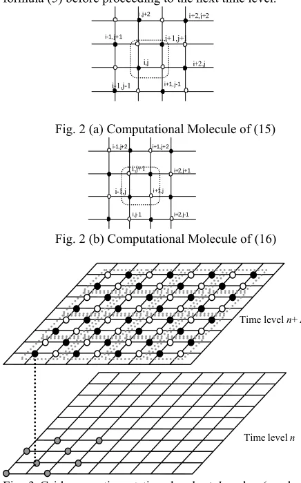
Referring to Fig. 2(a), it is observed that the iterative evaluation of (15) at any time level involves points of type only, while the evaluation of (16) involves points of type only (see Fig. 2(b)). Thus, the iterations may be chosen to involve only one type of points. Suppose we choose to iterate on points of type . Hence, the EDG scheme corresponds to generation of iterations on these points using the group formula (15) until a convergence test is satisfied. After convergence is achieved, the solutions at the points of type are evaluated directly once using the Crank-Nicolson formula (5) before proceeding to the next time level.

i+1,j+1

i,j

i ,j+2

i-1,j+1

i-1,j-1 i+1,j-1

i+2,j+2

i+2,j

Fig. 2 (a) Computational Molecule of (15)

i,j+1

i+1,j i+2,j+1 i+1,j+2 i-1,j+2

i-1,j

i,j-1 i+2,j-1

[image:3.612.68.286.366.716.2]

Fig. 2 (b) Computational Molecule of (16)

Fig. 3 Grid generation at time level n+1 and n (mesh size N=9)

IV. TRUNCATION ERROR AND CONSISTENCY

The local truncation for the Crank-Nicolson scheme may be obtained by using the Taylor series expansion about the point (xi, yj, tn+1/2):

2 3 2 2 2 2 2

3 2 2 2 2

, , 0.5 , , 0.5

2 2 4 3

2

2 2 4 3

, , 0.5 , , 0.5 , , 0.5 , , 0.5

4 3

2 4

, , 0.5

24 8

...

12 6

CN x y

i j n i j n

x x

x y

i j n i j n i j n i j n

y y

i j n

t u t u u

T a a

t t x t x

a b

u u u u

b b x

t x t y x x

a u b u

y y

+ +

+ + + +

+

⎛

Δ ∂ Δ _⎜ ∂ ∂ ∂ ∂

= − + _⎜ +

∂ _⎝ ∂ ∂ ∂ ∂

⎞ ⎛ ⎞

∂ ∂ ∂ ∂ _⎟ _⎜ ∂ ∂ _⎟

− − + _⎟+ Δ _⎜ − _⎟

∂ ∂ ∂ ∂ _⎠ _⎝ ∂ ∂ _⎠

∂ ∂

+Δ −

∂ 3

, , 0.5

2 2 2 4 2 3

2 4 2 3

, , 0.5 , , 0.5

2 2 2 4 2 3

2 4 2 3

, , 0.5 , , 0.5

48 2

...

48 2

i j n

x

i j n i j n

y

i j n i j n

y

a

x t u u

b

t x t x

a

y t u u

b

t y t y

+

+ +

⎛ ⎞

⎜ ⎟

⎜ ∂ ⎟

⎝ ⎠

⎛ ⎞

Δ Δ _⎜ ∂ ∂ ∂ ∂ _⎟

+ _⎜ − _⎟

∂ ∂ ∂ ∂

⎝ ⎠

⎛ ⎞

Δ Δ _⎜ ∂ ∂ ∂ ∂ _⎟

+ _⎜ − _⎟+

∂ ∂ ∂ ∂

⎝ ⎠

i.e. TCN = O(∆t2) + O(∆x2) + O(∆y2) (17)

Let h = ∆x = ∆y, k = ∆t, the local truncation error for this scheme is then

2 3

3

2 2 2 2 2 2 2

2 2 2 2 2 2

, , 0.5 , , 0.5 , , 0.5 , , 0.5

4 4 3 3

2

4 4 3 3

, , 0.5 , , 0.5 , , 0.5 , ,

24

...

8

12 12 6 6

CN

x y x y

i j n i j n i j n i j n

y y

x x

i j n i j n i j n i j n

k u

T t

k _a u _a u _b u _b u

t x t x t x t y

a b

a u u b u u

h

x y x y

+ + + +

+ + +

∂ = −

∂

⎛ _{∂ ∂} _{∂ ∂} _{∂ ∂} _{∂ ∂} ⎞

⎜ ⎟

+ _⎜ + − − + _⎟

∂ ∂ ∂ ∂ ∂ ∂ ∂ ∂

⎝ ⎠

∂ ∂ ∂ ∂

+ + − −

∂ ∂ ∂ ∂ 0.5

2 2 2 4 2 4 2 3 2 3

2 4 2 4 2 3 2 3

, , 0.5 , , 0.5 , , 0.5 , , 0.5

...

48 2 2

y x

x y

i j n i j n i j n i j n

a a

h k u u u u

b b

t x t y t x t y

+

+ + + +

⎛ ⎞

⎜ ⎟

⎝ ⎠

⎛ _{∂ ∂} _{∂ ∂} _{∂ ∂} _{∂ ∂} ⎞

⎜ ⎟

+ _⎜ + − − _⎟+

∂ ∂ ∂ ∂ ∂ ∂ ∂ ∂

⎝ ⎠

i.e. TCN = O(k2) + O(h2) . (18)

As ∆x, ∆y, ∆t → 0, the truncation error TCN tends to zero.

Hence, as the grid spacings ∆x, ∆y, ∆t →0 in the limit sense, the Crank Nicolson formula (5) is equivalent to the convection-diffusion equation and thus is consistent. EG is also consistent and its truncation error is similar with the Crank-Nicolson scheme since it is derived from the same formula.

Assuming that a = ax = ay, the truncation error for the

rotated Crank-Nicolson scheme becomes: 2 3

3

2 2 2 2 2 2 2

2 2 2 2 2 2

, , 0.5 , , 0.5 , , 0.5 , , 0.5

2 4 4 4

4 2 2 4

, , 0.5 , , 0.5 , , 0.5

24

...

8

2 12 2 12

R CN

x y

i j n i j n i j n i j n

i j n i j n i j n

k u

T

t

k u u u u

a a b b

t x t x t x t y

h a u a u a u

x x y y

−

+ + + +

+ + +

∂ = −

∂

⎛ _{∂ ∂} _{∂ ∂} _{∂ ∂} _{∂ ∂} ⎞

⎜ ⎟

+ + − − +

⎜ ∂ ∂ ∂ ∂ ∂ ∂ ∂ ∂ ⎟

⎝ ⎠

⎛ ∂ ∂ ∂

⎜

+ _⎜ + +

∂ ∂ ∂ ∂

⎝

3 3 3 3

3 2 3 2

, , 0.5 , , 0.5 , , 0.5 , , 0.5

2 2 2 4 2 4 2 4

2 4 2 2 2 2 4

, , 0.5 , , 0.5 , , 0.5

6 2 6 2

4

48 2 2

y y

x x

i j n i j n i j n i j n

i j n i j n i j n

x

b b

b u b u u u

x x y y x y

h k a u _a u a u

t x t x y t y

b

+ + + +

+ + +

⎞

∂ ∂ ∂ ∂ _⎟

− − − −

⎟

∂ ∂ ∂ ∂ ∂ ∂ _⎠

⎛ ∂ ∂ ∂ ∂ ∂ ∂

⎜

+ + +

⎜ ∂ ∂ ∂ ∂ ∂ ∂ ∂

⎝ ∂

− 2₂ 3₃ 2₂ 3 ₂ 2₂ 3₃ 2₂ 3₂

, , 0.5 , , 0.5 , , 0.5 , , 0.5

4_x _y 4_y ...

i j n i j n i j n i j n

u _b u _b u _b u

t x ₊ t x y ₊ t y ₊ t x y ₊

⎞

∂ ₋ ∂ ∂ ₋ ∂ ∂ ₋ ∂ ∂ _⎟₊

⎟

∂ ∂ ∂ ∂ ∂ ∂ ∂ ∂ ∂ ∂ _⎠

i.e. TR-CN = O(k2) + O(h2). (19)

Similarly, the rotated Crank-Nicolson equation (6) is consistent and the consistency of EDG is also maintained since it is based on the same formula.

V. STABILITY ANALYSIS

Explicit Group (EG)

Equation (8) can be written explicitly in difference form as un+1 = T un where T = A-1B. Here, Time level n+1

Time level n

ISBN: 978-988-18210-8-9

(4)

1 2

3 1 2

3 1

R R

R R R

A

R R R

R R ⎡ ⎤ ⎢ ⎥ ⎢ ⎥ ⎢ ⎥ = ⎢ ⎥ ⎢ ⎥ ⎢ ⎥ ⎣ ⎦ % % % , 1 3

2 1 3

1

2 1 3

2 1

G G

G G G

R

G G G

G G ⎡ ⎤ ⎢ ⎥ ⎢ ⎥ ⎢ ⎥ = ⎢ ⎥ ⎢ ⎥ ⎢ ⎥ ⎣ ⎦ % % %

,

5 2 5 G R G ⎡ ⎤ ⎢ ⎥ = ⎢ ⎥ ⎢ ⎥ ⎣ ⎦ %

,

4 3 4 G R G ⎡ ⎤ ⎢ ⎥ = ⎢ ⎥ ⎢ ⎥ ⎣ ⎦ %

,

1 0 0 0 0

a c e

b a e

G

d a c

d b a

− − ⎡ ⎤ ⎢₋ ₋ ⎥ ⎢ ⎥ = ⎢− − ⎥ ⎢ ₋ ₋ ⎥ ⎣ ⎦

,

2

0 0 0

0 0 0 0

0 0 0

0 0 0 0

b G b − ⎡ ⎤ ⎢ ⎥ ⎢ ⎥ =_⎢ _⎥ − ⎢ ⎥ ⎣ ⎦

,

3

0 0 0 0

0 0 0

0 0 0 0

0 0 0

c G c ⎡ ⎤ ⎢₋ ⎥ ⎢ ⎥ =_⎢ _⎥ ⎢ ₋ ⎥ ⎣ ⎦

,

4

0 0 0

0 0 0 0

d d G − ⎡ ⎤ ⎢ ₋ ⎥ ⎢ ⎥ = ⎢ ⎥ ⎢ ⎥ ⎣ ⎦

,

5

0 0 0 0

0 0 0

G e e ⎡ ⎤ ⎢ ⎥ ⎢ ⎥ = ⎢− ⎥ ⎢ ₋ ⎥ ⎣ ⎦ where 1

a= +Sx Sy+

,

2 4

Sx Cx

b= +

,

2 4

Sx Cx

c= −

,

2 4

Sy Cy

d= +

,

2 4 Sy Cy e= −

,

1 .

f= −Sx Sy−

= ( 1 0.5 0.25 0.5 0.25

0.5 0.25 0.5 0.25 ).

A Sx Sy Sx C x Sx C x

Sy C y Sy C y

∞

∴ + + + − + +

+ + + −

1 2

3 1 2

3 1

S S

S S S

B

S S S

S S ⎡ ⎤ ⎢ ⎥ ⎢ ⎥ ⎢ ⎥ = ⎢ ⎥ ⎢ ⎥ ⎢ ⎥ ⎣ ⎦ % % % , where 1 3

2 1 3

1

2 1 3

2 1

H H

H H H

S

H H H

H H ⎡ ⎤ ⎢ ⎥ ⎢ ⎥ ⎢ ⎥ = ⎢ ⎥ ⎢ ⎥ ⎢ ⎥ ⎣ ⎦ % % %

,

5 2 5 H S H ⎡ ⎤ ⎢ ⎥ = ⎢ ⎥ ⎢ ⎥ ⎣ ⎦ %

,

4 3 4 H S H ⎡ ⎤ ⎢ ⎥ = ⎢ ⎥ ⎢ ⎥ ⎣ ⎦

%

,

₁

0 0 0 0 f c e b f e H

d f c d b f

⎡ ⎤ ⎢ ⎥ ⎢ ⎥ = ⎢ ⎥ ⎢ ⎥ ⎣ ⎦

,

2

0 0 0

0 0 0 0 0 0 0 0 0 0 0

b H b ⎡ ⎤ ⎢ ⎥ ⎢ ⎥ = ⎢ ⎥ ⎢ ⎥ ⎣ ⎦

,

3

0 0 0 0 0 0 0 0 0 0 0

0 0 0

c H c ⎡ ⎤ ⎢ ⎥ ⎢ ⎥ = ⎢ ⎥ ⎢ ⎥ ⎣ ⎦

,

4

0 0 0

0 0 0 0 0 0 0 0 0 0 0

d d H ⎡ ⎤ ⎢ ⎥ ⎢ ⎥ = ⎢ ⎥ ⎢ ⎥ ⎣ ⎦

,

5

0 0 0 0 0 0 0 0 0 0 0

0 0 0

H e e ⎡ ⎤ ⎢ ⎥ ⎢ ⎥ = ⎢ ⎥ ⎢ ⎥ ⎣ ⎦

= ( 1 0.5 0.25 0.5 0.25

0.5 0.25 0.5 0.25 )

B Sx Sy Sx C x Sx C x

Sy Cy Sy C y

∞

∴ − − + − + +

+ + + −

1 1 1 ₁

T A B A B B

A

− −

∞ ∞ ∞ ∞ ∞

∞

∴ = ≤ ≤ ≤

for all Cx, Cy, Sx, Sy≥ 0. Therefore the EG iterative method is unconditionally stable.

Explicit Decoupled Group (EDG)

Equation (12) may also be expressed explicitly as un+1 =

T un where T = A-1B. The matrix A is of the form:

1 2

3 1 2

3 1

R R

R R R

A

R R R

R R ⎡ ⎤ ⎢ ⎥ ⎢ ⎥ ⎢ ⎥ = ⎢ ⎥ ⎢ ⎥ ⎢ ⎥ ⎣ ⎦ % % %

where 1 2

3 1 2

1

3 1 2

T

G G

G G G

R

G G G

⎡ ⎤ ⎢ ⎥ ⎢ ⎥ = ⎢ ⎥ ⎢ ⎥ ⎣ ⎦ % % %

,

3 43 4

2 3 4 3 G G G G R G G G ⎡ ⎤ ⎢ ⎥ ⎢ ⎥ ⎢ ⎥ = ⎢ ⎥ ⎢ ⎥ ⎢ ⎥ ⎣ ⎦ % %

,

2 5 2 3 5 2 5 2 T T T T G G G R G G G G ⎡ ⎤ ⎢ ⎥ ⎢ ⎥ ⎢ ⎥ = ⎢ ⎥ ⎢ ⎥ ⎢ ⎥ ⎣ ⎦ % %

,

1 a e G d a − ⎡ ⎤ = ⎢₋ ⎥ ⎣ ⎦ 2 0 0 0 G c ⎡ ⎤ = ⎢₋ ⎥ ⎣ ⎦ 3

0 0 0 G b ⎡ ⎤ = ⎢₋ ⎥ ⎣ ⎦ 4

0 0 0 G

e

⎡ ⎤

= ⎢_⎣₋ ⎥_⎦ 5

0

0 0

d G _{= ⎢}⎡ − ⎤_⎥

⎣ ⎦

with 1

2 2

Sx Sy

a= + +

,

4 8 8

Sx Cx Cy

b= + −

,

4 8 8

Sx Cx Cy

c= − +

,

4 8 8

Sy Cx Cy

d= + +

,

4 8 8

Sy Cx Cy

e= − −

,

1 .

2 2

Sx Sy

f= − −

= 1

2 2 4 8 8 4 8 8

.

4 8 8 4 8 8

A

Sx Cx Cy Sx Cx Cy

∞ ⎛ ∴ _⎜ + + + + − + − + ⎝ ⎞ + + + + − − _⎟ ⎠ 1 2

3 1 2

3 1

S S S S S B

S S S S S ⎡ ⎤ ⎢ ⎥ ⎢ ⎥ ⎢ ⎥ = ⎢ ⎥ ⎢ ⎥ ⎢ ⎥ ⎣ ⎦ % % %

,

where 1 2

3 1 2

1

3 1 2

T

H H H H H S

H H H

⎡ ⎤ ⎢ ⎥ ⎢ ⎥ = ⎢ ⎥ ⎢ ⎥ ⎣ ⎦ % % %

,

3 43 4

2 3 4 3 H H H H S H H H ⎡ ⎤ ⎢ ⎥ ⎢ ⎥ ⎢ ⎥ = ⎢ ⎥ ⎢ ⎥ ⎢ ⎥ ⎣ ⎦ % %

,

2 5 2 3 5 2 5 2 T T T T H H H S H H H H ⎡ ⎤ ⎢ ⎥ ⎢ ⎥ ⎢ ⎥ = ⎢ ⎥ ⎢ ⎥ ⎢ ⎥ ⎣ ⎦ % %

,

1 f e H d f ⎡ ⎤ = ⎢ ⎥

⎣ ⎦

,

2

0 0 0

H c

⎡ ⎤

= ⎢_⎣ ⎥_⎦

,

3

0 0 0 H b ⎡ ⎤ = ⎢ ⎥ ⎣ ⎦

,

4 0 0 0 H e ⎡ ⎤ = ⎢ ⎥

⎣ ⎦

,

5

0 0 0

d H _{= ⎢}⎡ ⎤_⎥

(5)

= 1

2 2 4 8 8 4 8 8

4 8 8 4 8 8

B

Sx Cx Cy Sx Cx Cy

∞

⎛

∴ _⎜ − − + + − + − +

⎝

⎞

+ + + + − − _⎟

⎠

Since the amplification matrix T=A-1_B,

1 1 1 ₁

T A B A B B A

− −

∞ ∞ ∞ ∞ ∞

∞

∴ = ≤ ≤ ≤

for all Cx, Cy, Sx, Sy≥ 0. Therefore, the EDG iterative scheme is unconditionally stable.

VI. NUMERICAL EXPERIMENTS

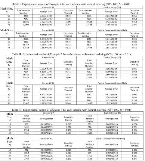
The experiments were carried out on a PC with Intel (R) Corel(TM)2 Duo CPU E7400 @ 2.80 GHz, 1.98 GB of RAM running Windows XP Pro using C compiler in Cygwin. Throughout the whole experiments, the absolute error test was used with tolerance equals to 10-10_{. One average error} was obtained at each time step. The Average Error depicted in Tables I-III denotes the maximum of all the average errors for the particular mesh size. Tables I, II and III present the numerical results of the four methods, the classical Crank-Nicolson, rotated point Crank-Nicolson, EG and EDG, in solving Examples 1, 2 and 3 respectively, for the number of time step NT = 100 and ∆t = 0.01.

Example 1(Diffusion problem)

We consider the following example (ax=ay=1, bx=by=0):

2 2

U U U t x y

∂ ∂ ∂

= +

∂ ∂ ∂

,

0≤ ≤x 1,0≤ ≤y 1,0≤ ≤t T.

The initial and boundary conditions are defined so that they satisfy the exact solution [3]:

(

) (

2

)

2

0.5 0.5

1

( , , ) exp , 0.

4 1 4 1 4 1

x y

U x y t t

t t t

⎧− − − ⎫

⎪ ⎪

= ₊ ⎨ ₊ − ₊ ⎬ >

⎪ ⎪

⎩ ⎭

₍₂₀₎

EG reduces the execution times up to 50% of the classical Crank-Nicolson while maintaining the same degree of accuracies. The execution timings of EDG are nearly 65% of the rotated Crank-Nicolson scheme. The latter was also observed to require lesser computing timings than the original Crank-Nicolson scheme.

Example 2

Consider the following example (ax = ay = bx = by = 1):

2 2

U U U U U

t x y x y

∂ ₌∂ ₊∂ ₋∂ ₋∂

∂ ∂ ∂ ∂ ∂

,

0≤ ≤x 1,0≤ ≤y 1,0≤ ≤t T The exact solution of the problem above is as follows [3]:

( ) (2 )2

0.5 0.5

1

( , , ) exp , 0.

4 1 4 1 4 1

x t y t

U x y t t

t t t

⎧− − − − − ⎫

⎪ ⎪

= ₊ ⎨ ₊ − ₊ ⎬ >

⎪ ⎪

⎩ ⎭

₍₂₁₎

Similar with Example 1, EG is faster than the Crank-Nicolson scheme, while EDG is faster than the rotated Crank-Nicolson and the EG schemes.

Fig. 4: Experimental Results of Example 1

Fig. 5: Experimental Results of Example 2 Example 3

We will consider a convection dominant problem. Let ax =

ay = 0.1, bx = by = 1.0, then the exact solution of the problem

above is denoted as below [3]:

(

)

(

)

(

)

2 2

0.5 0.5

1

( , , ) exp 10 10 , 0.

4 1 4 1 4 1

x t y t

U x y t t

t t t

⎧ _{− −} _{− −} ⎫

⎪ ⎪

= ₊ ⎨− ₊ − ₊ ⎬ >

⎪ ⎪

⎩ ⎭

(22) As shown in Table III and Fig. 6, EDG scheme requires the least execution timings compared to the other three methods. In all of the examples, the EG method produces almost the same accuracies as the classical Crank-Nicolson, while the EDG method is almost as accurate as the rotated Crank-Nicolson.

Fig. 6: Experimental results of Example 3 VII. CONCLUSIONS

In this paper, we have presented effective unconditionally stable group explicit iterative algorithms in solving the two dimensional convection-diffusion problem. The methods serve as viable alternative solvers to the problem with the group scheme derived from the rotated finite difference approximation requiring the least computing efforts among the schemes tested. The parallel implementation of these group methods are still under investigation and will be reported soon.

ISBN: 978-988-18210-8-9

(6)

REFERENCES

[1] A. R. Abdullah, “The Four Point Explicit Decoupled Group (EDG) Method: A Fast Poisson Solver,” International Journal of Comp. Math, vol. 38, 1991, pp. 61-70.

[2] N. M. Ali, The Design And Analysis of Some Parallel Algorithms For The Iterative Solution of Partial Differential Equations, PhD Thesis, Universiti Kebangsaan Malaysia, 1998.

[3] B.J. Noye, “Numerical Methods for Solving the Transport Equation, Numerical Modelling: Application to Marine Systems”, (ed. Noye), (Amsterdam: North Holland Publishing Company, 1987, 195-230). [4] W. S. Yousif and D. J. Evans, “ Explicit Group Over-relaxation

Methods for Solving Elliptic Partial Differential Equations,” Mathematics and Computers in Simulation, vol. 28, 1986, pp. 453-466. [5] W. S. Yousif and D. J. Evans, “Explicit DeCoupled Group Iterative

[image:6.612.69.551.141.676.2]

Methods and Their Parallel Implementations,” Parallel Algorithms and Applications, vol. 7, 1995, pp. 53-71.

Table I: Experimental results of Example 1 for each scheme with natural ordering (NT= 100, ∆t = 0.01) Mesh Size,

N

Classical C‐N Explicit Group (EG)

Total iteration

Number Average Error

Execution Time (s)

Total iteration

Execution Time (s) 13 3400 2.63323E‐04 0.031 2015 2.63323E‐04 0.016

21 7343 5.71861E‐05 0.125 4086 5.71848E‐05 0.063

37 19826 3.42176E‐05 1.109 10622 3.42213E‐05 0.453

49 32993 5.19494E‐05 3.297 17528 5.19566E‐05 1.360

Mesh Size, N

Rotated C‐N

Explicit Decoupled Group (EDG) Total iteration

Execution Time (s)

Total iteration

Execution Time (s)

13 2069 6.04169E‐04 0.015 1585 6.04169E‐04 0.015

21 4163 1.87250E‐04 0.031 3173 1.87250E‐04 0.031

37 10717 1.55451E‐05 0.313 8171 1.55443E‐05 0.219

49 17623 2.88300E‐05 0.922 13448 2.88311E‐05 0.610

Table II: Experimental results of Example 2 for each scheme with natural ordering (NT= 100, ∆t = 0.01) Mesh

Size, N

Total iteration Number

Average Error Execution Time (s)

13 3358 3.09292E‐04 0.031 2000 3.09292E‐04 0.016

21 7294 8.19951E‐05 0.141 4062 8.19938E‐05 0.063

37 19815 2.50416E‐05 1.141 10615 2.50448E‐05 0.485

49 33046 4.21901E‐05 3.406 17551 4.21967E‐05 1.438

Mesh Size,

N

Rotated C‐N

Explicit Decoupled Group (EDG) Total

iteration Number

Average Error Execution_Time_(s)

13 2056 6.87329E‐04 0.016 1583 6.87329E‐04 0.000

21 4144 2.24525E‐04 0.047 3169 2.24525E‐04 0.031

37 10710 3.32556E‐05 0.328 8185 3.32550E‐05 0.235

49 17647 1.99782E‐05 0.969 13497 1.99791E‐05 0.641

Table III: Experimental results of Example 3 for each scheme with natural ordering (NT= 100, ∆t = 0.01) Mesh

Size, N

13 905 0.010664914 0.016 675 0.010664914 0.000

21 1431 0.004067973 0.031 966 0.004067973 0.031

37 2954 0.001327565 0.188 1789 0.001327564 0.094

49 4551 0.000783234 0.500 2631 0.000783233 0.234

Mesh Size, N

Rotated C‐N

Explicit Decoupled Group (EDG) Total

iteration Number

13 742 0.020605961 0.016 588 0.020605961 0.016

21 1064 0.007780534 0.016 819 0.007780534 0.016

37 1918 0.002522236 0.078 1465 0.002522363 0.063