3813
On Knowledge Distillation from Complex Networks for Response
Prediction
Siddhartha Arora1,2 and Mitesh M. Khapra1,2 and Harish G. Ramaswamy1,2 1Department of Computer Science and Engineering, Indian Institute of Technology Madras
2Robert Bosch Centre for Data Science and AI (RBC-DSAI),
Indian Institute of Technology Madras
{sidarora,miteshk,hariguru}@cse.iitm.ac.in
Abstract
Recent advances in Question Answering have lead to the development of very complex mod-els which compute rich representations for query and documents by capturing all pair-wise interactions between query and docu-ment words. This makes these models ex-pensive in space and time, and in practice one has to restrict the length of the docu-ments that can be fed to these models. Such models have also been recently employed for the task of predicting dialog responses from available background documents (e.g., Holl-E dataset). However, here the documents are longer, thereby rendering these complex mod-els infeasible except in select restricted set-tings. In order to overcome this, we use stan-dard simple models which do not capture all pairwise interactions, but learn to emulate cer-tain characteristics of a complex teacher net-work. Specifically, we first investigate the conicity of representations learned by a com-plex model and observe that it is significantly lower than that of simpler models. Based on this insight, we modify the simple archi-tecture to mimic this characteristic. We go further by using knowledge distillation ap-proaches, where the simple model acts as a student and learns to match the output from the complex teacher network. We experiment with the Holl-E dialog data set and show that by mimicking characteristics and matching out-puts from a teacher, even a simple network can give improved performance.
1 Introduction
The advent of large scale datasets for QA has lead to the development of increasing complex neural models with specialized components for (i) en-coding the query (ii) enen-coding the document(s) (iii) capturing interactions between document and query words and (iv) generating/extracting the correct answer span from the given document (Seo et al.,2016;Hu et al.,2017;Yu et al.,2018). While
these models give state-of-the-art performance on a variety of datasets, they have very high space and time complexity. This is a concern, and in prac-tice, it is often the case that one has to resort to restricting the maximum length of the input docu-ment such that the model can run with reasonable resources (say, a single 12GB Tesla K80 GPU).
Such complex span prediction models are also being adapted for other NLP tasks such as dialog response prediction (Moghe et al.,2018), which is the focus of this work. In particular, we refer to theHoll-Edataset where the task is to extract the next response from a document which is relevant to the conversation (see Figure1). This setup is very similar to QA wherein the input is{context, document}as opposed to {query, document}and the correct response span needs to be extracted from the given document. Given this similarity, it is natural to adopt existing QA models (Seo et al.,
2016;Yu et al.,2018) for this task. However, the documents in Holl-E dataset are longer, and the authors specifically report that they were unable to run these models when the entire document was given as input. Hence, they report results only in constrained oracle settings where the document is trimmed such that the response still lies in the shortened document. The above situation suggests that there is clearly a trade-off needed. On one hand, we want to harness the power of these com-plex models to achieve better performance and on the other hand we want to be able to run them with reasonable compute resources without arbitrarily trimming the input document.
cap-Source Doc: ...comes in. As soon as the door is open, the Bride’s fist crashes into Vernita’s face. A savage fight follows, first with fists, then with knives.... The fight pauses ... At this point Vernita is introduced as a member of the Deadly Vipers, codename Copperhead. ...
Sample Conversation:
Prober (S1):Which is your favourite character in this?
Responder (S2): My favorite character was Copperhead because she was kicking butt.
Prober (S3): Oh my goodness I agree, because the fight with Vernita was the best in the whole movie.
Responder (S4): It’s starts off action packed because
as soon as the door is open, the Bride’s fist crashes into Vernita’s face. A savage fight follows, first with fists, then with knives.
Prober (S5):And it gets better when we find out they are both assassins.
Responder (S6): And a group of them, Vernita is introduced as a member of the Deadly Vipers, codename Copperhead.
Figure 1: Sample Conversation from the Holl-E Dataset. Note that the underlined responses directly correspond to spans in the background document.
tured, the model computes a final representation which is then fed to a decoder to predict the cor-rect span in the document. This recipe is very sim-ilar to BiDAF (Seo et al.,2016), QANeT (Yu et al.,
2018) but the main difference is that these models use much more complex encoder and interaction components to arrive at the final representation. As expected, the performance of this model is poor when compared to BiDAF, QANeT. The aim now is to improve the performance of this model by carefully analysing or learning from complex models. Given that the complex model differs in the manner in which the final representation is computed, one hypothesis is that it learns richer fi-nal representations than the simple model. Indeed, on investigation, we found that the final represen-tations learned by complex models are diverse for different inputs (context, document pairs) as com-pared to the simple model. Based on this insight, we propose a modification to the simple model which increases the diversity of the embeddings, thereby improving the performance.
While this insight obtained by manual investi-gation is useful, there is clearly scope for learn-ing by explorlearn-ing other characteristics of the model. One principled way of doing this is to use knowl-edge distillation (Hinton et al., 2015) where the simple model acts as a student and learns to mimic the probability distributions predicted by a teacher. In other words, instead of simply maximizing the log likelihood of the training data, the simple
model now gets additional signals from the teacher which act as hints while training.
Our experiments, using theHoll-Edataset show that by (i) improving the conicity (Chandrahas et al.,2018) of the representations learned by the simple model and (ii) mimicking the outputs of the complex teacher model the simple model can give improved performance with fewer compute and memory requirements. In particular, when com-pared to a standalone simple model the student model shows an improvement of3.4% (compare SAM-mul-train (LD) and SAM-add-topk (LD) en-tries in Table2and Table3respectively).
2 Related Work
Over the past few years neural sequence predic-tion models which take a quespredic-tion as input and predict the corresponding answer span in a given document have evolved rapidly. Such models have also been adapted for dialog response predic-tion in the context of the Holl-Edataset (Moghe et al., 2018). These models typically differ in the components used for capturing interactions between query and document, capturing interac-tions between sentences in a document and refin-ing the query/document representation over multi-ple passes (Shen et al.,2017;Dhingra et al.,2017;
Sordoni et al.,2016).
In particular, a co-attention network which computes the importance of every query word w.r.t. every document word and the importance of every document word w.r.t. every query word is an important component in most state of the art mod-els (Hermann et al.,2015;Kadlec et al.,2016;Cao et al., 2016;Xiong et al., 2016;Seo et al., 2016;
Gong and Bowman, 2017;Dhingra et al., 2017;
Wang et al., 2017; Shen et al., 2017; Trischler et al., 2016; Group and Asia, 2017; Tan et al.,
2017;Sordoni et al.,2016). Similarly, some mod-els (Group and Asia, 2017;Seo et al., 2016;Hu et al.,2017) contain a self-attention network which computes the importance of every document word w.r.t. every other document word. In general, the most successful models (for example, BiDAF (Seo et al.,2016), QANeT (Yu et al.,2018)) use a combination of these components which capture all pairwise interactions and are thus computation-ally very expensive. As a result, in practice, these models are not suitable for longer documents.
compact models (Cheng et al., 2017). For exam-ple,Ba and Caruana(2014);Hinton et al.(2015);
Lopez-Paz et al.(2016);Chen et al.(2017) train a shallow student network using soft targets (or class probabilities) generated by an expensive teacher instead of the hard targets present in the training data.Romero et al.(2015) extend this idea to train a student model using the intermediate represen-tations learned by the teacher model which act as additional hints. This idea of Knowledge Distil-lation has also been tried in the context of prun-ing networks for multiple object detection (Chen et al.,2017), speech recognition (Wong and Gales,
2016). In the context of reading comprehension or span prediction,Hu et al.(2018) have very re-cently shown that we can distill knowledge from an ensemble of models into a single model. How-ever, unlike our work, the single model itself is a complex model (Hu et al., 2017) containing an expensive self attention network and a RL agent. To the best of our knowledge, ours is the first work which tries to build a simple span prediction model by distilling knowledge from a complex model.
3 Models For Response Prediction
We view a conversation as sequence of utterances by aproberand aresponder. The response predic-tion (RP) model aims to predict the utterance by the responder based on a source document, when given the query (prober’s most recent utterance) and the history (past utterance by the prober and responder). See Figure1for an example.
We denote the lengths of source document, query, prober history and responder history as
T, I, J, K. The LSTMs/GRUs used all have the same number of cells, denoted byd. In particu-lar, the document lengthT is of the order of a few thousands and the query/history lengths I, J, K
are of the order of a few hundreds. Contrast this with QA tasks, whereT is only of the order of a few hundreds, and the query length (I+J+K) is of the order of a few tens.
3.1 BiDAF for RP
BiDAF (Seo et al.,2016) is an extremely popular model used for span prediction in reading compre-hension based question answering problems. We can frame the problem of response prediction as one of question answering by concatenating the query, prober history, and responder history into a
single “question”. BiDAF has proven to be hugely successful in QA tasks, but has a large number of parameters (about 2.5 million) and consumes a large amount of computational space and time during training and prediction.
We use the BiDAF model as a guiding post while constructing our model, and in particular focus on the so calledquery to context attention, which is a vector (denoted byeh) that indicates the
weighted sum of the most important words in the source document, with respect to the query and histories.
3.2 QANeT for RP
QANeT (Yu et al.,2018) is another recent model used for span prediction in QA tasks and specifi-cally targets better space and time efficiency than BiDAF. Despite this, it still has a large number of parameters (about 1.3 million) and still consumes a large amount of computational space and time during training and prediction. The QANeT model can also be modified for response prediction in a similar manner to BiDAF.
3.3 Simple Attention Model for RP
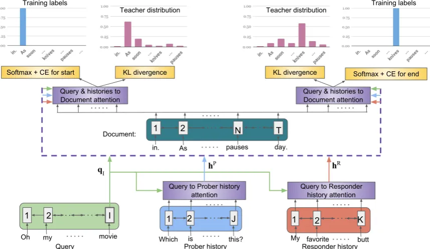
We now describe the simple attention model that we aim to learn. In a fashion similar to that of BiDAF and QANeT architectures, the simple model also operates in 3 distinct layers. See Fig-ure2for an overview into the model.
3.3.1 Word Embedding Layer
The words from the source document, the utter-ances by the prober and the responder are all en-coded using standard GloVe embeddings ( Pen-nington et al.,2014).
3.3.2 Contextual Embedding Layer
In the next layer we encode the query (prober’s most recent utterance) using a BiGRU/BiLSTM, and encode the previous utterances of the prober and responder in a query sensitive manner.
Query Encoder: Embedded query words are passed through BiGRU where final stateqI ∈R2d
acts as query representation.
Query Sensitive History Summariser: The history of the prober and responder are passed through a BiGRU to get context sensitive vectors hPj ∈R2dandhR
k ∈R2dforj∈[J]andk∈[K].
These vectors are combined to get vectors hP
Query to Prober history attention
Query to Responder history attention qI
is
Which this?
Softmax + CE for start Softmax + CE for end
.
As
in. pauses
Query & histories to Document attention
Query & histories to Document attention
hP hR
1 J 1 2
1 2 I 2
My favorite butt
1 2 K
1 2 T
Oh my movie
day.
N
1 2 I
Teacher distribution Teacher distribution
Training labels Training labels
KL divergence KL divergence
Query Prober history Responder history
[image:4.595.79.508.66.314.2]Document:
Figure 2: A Simple Attention Model with (1) Query Encoder, Prober History Encoder, Responder History Encoder, and Document Encoder (2) Query to Prober History Attention, Query to Responder History Attention, and Query & histories to Document Attention (3) Training Labels and Teacher Distribution.
be viewed as query-aware representations of the prober and responder history. The equations for hP are given below. The vectorhR is also
calcu-lated in a similar manner.
ej = mulW P
(hPj,qI)
α= softmax(e)
hP=X j
αjhPj
wheremulW(v0,v1) = v>0Wv1 is a
parameter-ized multiplicative way of capturing the interac-tion between two vectors.
3.3.3 Span Prediction Layer
The source document is finally used in this layer to predict the start and end indices of the response. The GloVe embedded words of the source docu-ment are passed through a BiGRU to get context sensitive vectorsut ∈ R2d, for allt ∈ [T]. Each
indextgets a scorestbased on the interaction
be-tweenutand the query/history vectorsqI,hP,hR.
The scoresstare normalized by a softmax and is
taken to be the prediction of the starting word in-dex.
st= mulW strt
(ut,qI,hP,hR)
α= softmax(s)
wheremulW(u0, . . . ,ua) =u>0 Pa
i=1Wiui
A similar method is used for the prediction of the ending word index as well.
4 Bridging The Gap Between Simple and Complex Models
We performed several experiments on the Holl-E dataset and observed that the complex mod-els (QANeT and BiDAF) perform better than the simple attention model described in Section 3.3. However, they take significantly more time and memory for training and inference. In fact, for the examples with longer source documents, both BiDAF and QANeT run into memory issues when training. During prediction, the memory issues in QANeT and BiDAF can be sidestepped by break-ing the source document into multiple chunks and taking the highest scoring span.
In the rest of this section we study several approaches to nudge the simple attention model to take parameters that make it have similar be-haviour as the complex models, and check if the so nudged model demonstrates better performance on the Holl-E dataset.
4.1 Diversity of Embeddings
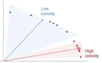
Figure 3: Conicity (i.e., average cosine similarity of vectors with the mean of all the vectors) of two sets of vectors with standard deviation 0.1 (red) and 1.3 (blue)
same conversation are often the same, even though the “right response” is different in those points. For example, consider the conversation in Figure
1. We expect the trained model to be such that
Pred span(SD, S1, S2, S3) =spanSD(S4)
whereSDis the source document, andSi are the
the utterances in the conversation. Similarly, we expect the trained model to be such that
Pred span(SD, S3, S4, S5) =spanSD(S6)
However we often find that our simple model pre-dicts the same span for both the cases above, which is wrong (unlessS4 andS6 are the same.)
We hypothesize this as being due to the context sensitive embeddings of the history not depend-ing strongly on the query, and hence the span pre-diction model picks up most information from the source document. To support this point of view we measured the diversity of the context-to-query vectorshe of the BiDAF model for several
exam-ples grouped by conversation. In more detail we computed theconicity(Chandrahas et al.,2018) of vectorshe(SD, S1, S2, S3),eh(SD, S3, S4, S5), . . .
for every conversation in the test set and averaged it over all conversations. (See Figure 3 for an overview on conicity). This average conicity was observed to be about0.6(see Table6), which, ac-cording toChandrahas et al. (2018), is low (low conicity implies high diversity).
We observe similar behaviour for QANeT as well. The average conicity of the row sums of thesimilarity matrixgrouped by conversation was also observed to be about0.6(see Table6).
On the other hand, for our simple attention model, the average conicity of the vectorshRand hP, when computed in a similar fashion as
men-tioned above were generally high (about0.8) (see Table6).
Based on these observations we hypothesize that decreasing the conicity of the vectorshR and hP would improve the performance of the sim-ple attention model. In particular, we propose to change the multiplicative method of combining vectors into an additive method instead.
In particular we propose to replace the function
mul in our simple model with the function add
defined as follows:
addW(v0,v1, . . . ,va) =w>tanh a
X
i=0 Wivi
!
where the vectorw and the matrices Wi param-eterize the mode of combining the input vectors. This is motivated byChandrahas et al.(2018) who show that using additive model in embedding of entities in knowledge graphs gives consistently better diversity than using multiplicative models.
4.2 Standard Knowledge Distillation from Complex Models
While borrowing high level ideas from complex models, like increasing diversity of the learned representation can help to some extent, one can push this further to distill the learned complex model (Hinton et al.,2015) into the simple atten-tion model. To achieve this, we train a teacher model (BiDAF or QANeT) on the training set and use it to make predictions on the same training set. The simple attention model would minimise the sum of two loss functions: 1) Cross entropy loss of the predicted start and end indices with the train labels of the start and end indices, 2) KL-divergence of the predicted start and end indices from the teacher prediction of the same. The loss on a single training sample is given below
D(pTb||pSb) +D(yb||pSb) +D(pTe||pSe) +D(ye||pSe)
(1) where D denotes the KL divergence, pT
b,pTe
de-note the predicted begin index and end index dis-tribution of the teacher model, andpSb,pSe denote the predicted begin and end index distribution of the student model andyb,ySdenote the true begin
and end index in one-hot vector form.
4.3 Top-kBased Knowledge Distillation
on a single training sample is given below
D(pe T b||ep
S
b) +D(yb||pSb) +D(pe T e||pe
S
e) +D(ye||pSe)
(2) whereep
T b,pe
T
e gives just the (normalised)
probabil-ity of the top-kpredictions of teacher model on the begin and end indices. SimilarlypeS
b,pe S
e gives the
student predictions for the begin and end indices restricted to the top-kentries given by the teacher model.
4.4 Other Knowledge Distillation Approaches
As the teacher model is already trained, and the main objective in knowledge distillation is to have the student model mimic the teacher model, there is no need to restrict the objective terms 1 and 3 in equation1to only the training data. Hence by hallucinating conversations and documents we can get more terms in the objective and has an effect similar to data augmentation.
Another possible way to take advantage of teacher models is to extract more information than simply the predicted spans for each training exam-ple from the teacher models. In particular one easy way to extract piece of information is the gradient of the model output with respect to the input for the teacher model. The so called Sobolev training (Czarnecki et al.,2017) exploits this information and adds two more extra terms to the objective in (1).
||∇pTb − ∇pSb||2+||∇pTe − ∇pSe||2
The gradients are all taken with respect to the model input, which would be the source docu-ment, the query and the histories.
5 Experiments
In this section, we describe the setup used for our experiments and discuss the results.
5.1 Experiment Setup
We perform experiments using the Holl-E conver-sation dataset (Moghe et al.,2018) which contains crowdsourced conversations from the movie do-main. Every conversation in this dataset is asso-ciated with background knowledge comprising of plot details (from Wikipedia), reviews and com-ments (from Reddit). Every alternate utterance in the conversation is generated by copying and/or
modifying sentences from this unstructured back-ground knowledge. We refer the reader again to Figure1for a sample from this dataset.
We use the same train, test and validation splits as provided by the authors of the original paper (Moghe et al.,2018). For each chat in the train-ing data, the authors construct traintrain-ing triplets of the form{document, context, response}where the number of train, test and validations triplets are 34486, 4388 and 4318 respectively. The context contains (i) the query (the prober’s most recent ut-terance) and (ii) the history (past 2 utterances by the prober and the responder) as described earlier. The task then is to train a model which can predict the response given the document and the context. At test time, the model is shown document, con-text and predicts the response.
As mentioned earlier, the authors of Holl-E found that BiDAF and QANeT run into memory issues when evaluated on their dataset. Hence, they propose two setups (i) long document (LD) setup and (ii) short document (SD) setup. In the long document setup, the authors do not trim the document from which the response needs to be predicted. In the short document setup, the au-thors trim the document to 256 words such that the span containing the response is contained in the trimmed document. This enables them to evalu-ate BiDAF and QANeT on the trimmed document. We also report experiments using both the LD and SD setup.
As mentioned above complex models (BiDAF and QANeT) face memory issues on training set with long documents. So for all situations where we need predictions from complex models for long documents, we use a BiDAF/QANeT model trained on short document examples, and the pre-diction on the long document is made by splitting the long documents into chunks and feeding it to the trained BiDAF/QANeT model. The final pre-dicted span is the largest scoring span across all chunks.
For all models, we considered the following hy-perparameters and tuned them using the validation set. We tried batch sizes of 32 and 64 and the following GRU sizes: 64, 100, 128. We experi-mented with 1, 2 and 3 layers of GRU. We used pre-trained publicly available Glove word embed-dings1of 100 dimensions. The best performance
1https://nlp.stanford.edu/projects/
SAM, SD SAM, LD BiDAF, SD BiDAF, LD QANeT, SD QANeT, LD
Memory 540MB 1.3GB 11GB 11GB 3GB 3GB
Time 30 secs 43 sec 347 secs 710 secs 90 secs 150 secs
Table 1: ‘Inference’ Memory and Time usage for different models. Here SAM, SD and LD refers to Simple Attention Model, short document and long document respectively.
Model LD SD
SAM-mul-train 36.49 40.08 SAM-add-train 36.96 41.30
BiDAF 38.30* 45.54
[image:7.595.88.506.61.107.2]QANeT 38.10* 47.67
Table 2: Performance (F1 Scores) of different baseline models on SD (short document) and LD (long document) test set.
Model Details BiDAF QANeT
SAM-mul 36.50 37.03
SAM-add 37.14 37.28
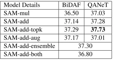
SAM-add-topk 37.29 37.73
SAM-add-aug 37.17 37.01
SAM-add-ensemble 37.30
SAM-add-both 36.80
Table 3: F1 Scores for different variants of simple attention model on long documents test set.
was with the batch size of 32, 2 layers of GRU with hidden size 64. We used Adam (Kingma and Ba,2014) optimizer with initial learning rate set to
0.001, β1 = 0.9, β2 = 0.999. We performed L2
weight decay with decay rate set to0.001.
5.2 Model Variant Details
The models that we experiment with are listed below:
1. SAM-add-Train: The simple attention model with additive interactions and no teacher terms in the objective (Only terms 2 and 4 in Eqn. (1)). 2. SAM-add-Teach: The simple attention model with additive interactions and only knowledge dis-tillation terms in the objective (Only terms 1 and 3 in Eqn. (1)).
3. SAM-add : The simple attention model with additive interactions and both knowledge distilla-tion terms and training data terms in the objective (all terms in1).
4. SAM-add-topk : The simple attention model with additive interactions and knowledge distilla-tion applied to the top-kindices and training data terms in the objective (all terms in2).
5. SAM-add-aug: The SAM-add model, where the teacher terms are evaluated on hallucinated data in addition to training data. The halluci-nated data are derived from the original training set by reordering the words in the source docu-ment, query and histories.
6. SAM-add-grad : The SAM-add model, with extra terms in the loss penalising the deviation of the gradient of the simple model from the gradient
of the teacher model.
7.SAM-add-both: Same as the SAM-add model, but has 6 terms instead of the 4 terms in Equa-tion1. The extra two terms arise from usingboth QANeT and BiDAF instead of just one.
8. SAM-add-ensemble : Same as the SAM-add model, but the teacher predictions pT are set as the average of the QANeT and BiDAF predictions.
All the “add” models above also have a “mul” variant where the additive interaction add is re-placed by a multiplicative interactionmul.
5.3 Results and Discussion
The F1-scores of the various models we train are given in Table 2, Table 3 and Table 4. A sum-mary of the space and time complexity of predic-tion with the simple model and the complex mod-els is given in Table1. The training times and pa-rameter counts of the models are given in Table5
We draw several conclusions and inferences from these results and make some comments below. Efficient Training with Simple Model:From Ta-ble5, we observe that simple attention model has 5 to 10 times less parameters than QANeT and BiDAF. The training time of the simple model is also significantly lesser than that of the complex models.
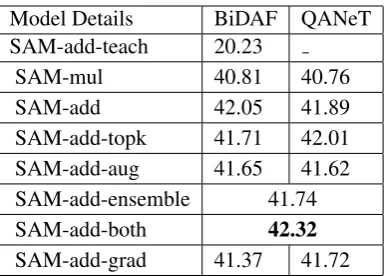
[image:7.595.313.506.149.251.2] [image:7.595.81.244.153.226.2]Model Details BiDAF QANeT SAM-add-teach 20.23
SAM-mul 40.81 40.76
SAM-add 42.05 41.89
SAM-add-topk 41.71 42.01
SAM-add-aug 41.65 41.62
SAM-add-ensemble 41.74
SAM-add-both 42.32
SAM-add-grad 41.37 41.72
Table 4: F1 Scores for different variants of simple attention model on short document test set.
SAM BiDAF QANeT
[image:8.595.75.269.60.198.2]Parameters 0.25 M 2.5 M 1.3 M Train Time 307 secs 5880 secs 2213 secs
Table 5: Comparison of parameters (in Million) and training time (seconds) per epoch for different models.
Model Conicity
Complex Models 0.6
SAM-mul 0.8
SAM-add 0.7
Table 6: Comparison of conicity between variants of simple-attention model and complex models.
model by splitting the source document into man-ageable chunks.
Conicity of Multiplicative models vs Additive Models: As noted before we use two distinct methods to capture the interaction between a group of vectors : an additive mechanismadd, and a multiplicative mechanism mul. As mentioned earlier, an additive model for capturing interac-tions has been hypothesized to increase diversity. This is true in our case as well: the conicity of the hP andhR vectors goes down from about 0.8 to
0.7 (compare SAM-mul and SAM-add entries in Table6) when using the additive model instead of the multiplicative model.
F1 scores of Multiplicative models vs Additive Models: In addition to improving diversity, us-ing the additive modeladd instead of the multi-plicative modelmulincreases F1-scores all across the board. We have not reported scores for certain multiplicative variants because their performance is significantly worse.
F1 scores of Simple Model with Knowledge Dis-tillation: We observe that using a teacher model for knowledge distillation using the objective in (1) almost always improves the performance of the simple model.
Importance of training labels: The objective in knowledge distillation (Equation (1)) involves both the training labels and the teacher predicted distribution. Even though the teacher predicted distribution also incorporates the training data, re-moving the training data term from the objective of knowledge distillation worsens performance significantly.
Top-k Distillation: The knowledge distillation approach based on top-kpredicted indices results in the best simple model for long document
exam-ples (see Table3). The value of k was chosen to be 50 for the short document case and it is 20 for the long document case.
Add-Both Knowledge Distillation: Learning from multiple teachers could lead to better perfor-mance hence we trained the student model with two teachers (BiDAF+QANeT). Here the objec-tive function of student is to minimize KL Diver-gence between predictions for both teachers. We achieved best results with this technique on short document (SD) test set.
Data Augmentation and Gradient Distillation: While the data augmentation and gradient distilla-tion methods hold a lot of promise, in the experi-ments that we conducted, we did not see a signifi-cant improvement.
QANeT Teachers vs BiDAF Teachers:Using ei-ther QANeT or BiDAF as a teacher doesn’t seem to make any difference in the performance of the student models (compare the two columns in Table
3and4).
6 Conclusion
[image:8.595.291.514.63.105.2]model. We experimented with the Holl-E conver-sation dataset and showed that by mimicking char-acteristics of the teacher a simple model can give improved performance.
Acknowledgements
We thank Department of Computer Science and Engineering, and Robert Bosch Center for Data Sciences and Artificial Intelligence, IIT Madras (RBC-DSAI) for providing us with adequate com-pute resources. Lastly, we thank Ananya Sai and Shweta Bhardwaj for valuable discussions and re-viewing intial drafts of this paper.
References
Jimmy Ba and Rich Caruana. 2014. Do deep nets really need to be deep? InAdvances in Neural Information Processing Systems 27, pages 2654–2662.
Ziqiang Cao, Wenjie Li, Sujian Li, Furu Wei, and Yan-ran Li. 2016. Attsum: Joint learning of focusing and summarization with neural attention. In COLING, pages 547–556. ACL.
Chandrahas, Aditya Sharma, and Partha P. Talukdar. 2018. Towards understanding the geometry of knowledge graph embeddings. In Proceedings of the 56th Annual Meeting of the Association for Com-putational Linguistics, ACL 2018, Melbourne, Aus-tralia, July 15-20, 2018, Volume 1: Long Papers, pages 122–131.
Guobin Chen, Wongun Choi, Xiang Yu, Tony Han, and Manmohan Chandraker. 2017. Learning efficient object detection models with knowledge distillation. In I. Guyon, U. V. Luxburg, S. Bengio, H. Wallach, R. Fergus, S. Vishwanathan, and R. Garnett, editors, Advances in Neural Information Processing Systems 30, pages 742–751. Curran Associates, Inc.
Yu Cheng, Duo Wang, Pan Zhou, and Tao Zhang. 2017. A survey of model compression and acceleration for deep neural networks. CoRR, abs/1710.09282.
Wojciech Marian Czarnecki, Simon Osindero, Max Jaderberg, Grzegorz Swirszcz, and Razvan Pascanu. 2017. Sobolev training for neural networks. CoRR, abs/1706.04859.
Bhuwan Dhingra, Hanxiao Liu, Zhilin Yang, William W. Cohen, and Ruslan Salakhutdinov. 2017. Gated-attention readers for text comprehen-sion. In Proceedings of the 55th Annual Meeting of the Association for Computational Linguistics, ACL 2017, Vancouver, Canada, July 30 - August 4, Volume 1: Long Papers, pages 1832–1846.
Yichen Gong and Samuel R. Bowman. 2017. Rumi-nating reader: Reasoning with gated multi-hop at-tention. CoRR, abs/1704.07415.
Natural Language Computing Group and Mi-crosoft Research Asia. 2017. R-net: Machine reading comprehension with self-matching net-works. ACL, abs/1606.02245.
Karl Moritz Hermann, Tom´as Kocisk´y, Edward Grefenstette, Lasse Espeholt, Will Kay, Mustafa Su-leyman, and Phil Blunsom. 2015. Teaching ma-chines to read and comprehend. In Advances in Neural Information Processing Systems 28: Annual Conference on Neural Information Processing Sys-tems 2015, December 7-12, 2015, Montreal, Que-bec, Canada, pages 1693–1701.
Geoffrey Hinton, Oriol Vinyals, and Jeffrey Dean. 2015. Distilling the knowledge in a neural network. InNIPS Deep Learning and Representation Learn-ing Workshop.
Minghao Hu, Yuxing Peng, and Xipeng Qiu. 2017. Mnemonic reader for machine comprehension. CoRR, abs/1705.02798.
Minghao Hu, Yuxing Peng, Furu Wei, Zhen Huang, Dongsheng Li, Nan Yang, and Ming Zhou. 2018. Attention-guided answer distillation for machine reading comprehension. In EMNLP, pages 2077– 2086. Association for Computational Linguistics.
Rudolf Kadlec, Martin Schmid, Ondrej Bajgar, and Jan Kleindienst. 2016. Text understanding with the at-tention sum reader network. In Proceedings of the 54th Annual Meeting of the Association for Compu-tational Linguistics, ACL 2016, August 7-12, 2016, Berlin, Germany, Volume 1: Long Papers.
Diederik P. Kingma and Jimmy Ba. 2014. Adam: A method for stochastic optimization. CoRR, abs/1412.6980.
D. Lopez-Paz, B. Sch¨olkopf, L. Bottou, and V. Vapnik. 2016. Unifying distillation and privileged informa-tion. InInternational Conference on Learning Rep-resentations.
Nikita Moghe, Siddhartha Arora, Suman Banerjee, and Mitesh M. Khapra. 2018. Towards exploiting back-ground knowledge for building conversation sys-tems. In Proceedings of the 2018 Conference on Empirical Methods in Natural Language Process-ing, Brussels, Belgium, October 31 - November 4, 2018, pages 2322–2332.
Jeffrey Pennington, Richard Socher, and Christo-pher D. Manning. 2014. Glove: Global vectors for word representation. In Proceedings of the 2014 Conference on Empirical Methods in Natural Lan-guage Processing, EMNLP 2014, October 25-29, 2014, Doha, Qatar, A meeting of SIGDAT, a Special Interest Group of the ACL, pages 1532–1543.
Min Joon Seo, Aniruddha Kembhavi, Ali Farhadi, and Hannaneh Hajishirzi. 2016. Bidirectional at-tention flow for machine comprehension. CoRR, abs/1611.01603.
Yelong Shen, Po-Sen Huang, Jianfeng Gao, and Weizhu Chen. 2017. ReasoNet: Learning to Stop Reading in Machine Comprehension. In KDD, pages 1047–1055. ACM.
Alessandro Sordoni, Phillip Bachman, and Yoshua Bengio. 2016. Iterative alternating neural attention for machine reading. CoRR, abs/1606.02245.
Chuanqi Tan, Furu Wei, Nan Yang, Weifeng Lv, and Ming Zhou. 2017. S-net: From answer extraction to answer generation for machine reading comprehen-sion.CoRR, abs/1706.04815.
Adam Trischler, Zheng Ye, Xingdi Yuan, Philip Bach-man, Alessandro Sordoni, and Kaheer Suleman. 2016. Natural language comprehension with the epireader. In EMNLP, pages 128–137. The Asso-ciation for Computational Linguistics.
Wenhui Wang, Nan Yang, Furu Wei, Baobao Chang, and Ming Zhou. 2017. Gated self-matching net-works for reading comprehension and question an-swering. InProceedings of the 55th Annual Meet-ing of the Association for Computational LMeet-inguis- Linguis-tics, ACL 2017, Vancouver, Canada, July 30 - August 4, Volume 1: Long Papers, pages 189–198.
Jeremy H. M. Wong and Mark J. F. Gales. 2016. Se-quence student-teacher training of deep neural net-works. In Interspeech 2016, 17th Annual Confer-ence of the International Speech Communication As-sociation, San Francisco, CA, USA, September 8-12, 2016, pages 2761–2765.
Caiming Xiong, Victor Zhong, and Richard Socher. 2016. Dynamic coattention networks for question answering.CoRR, abs/1611.01604.