A Semantic Scattering Model for the Automatic Interpretation of Genitives

A Semantic Scattering Model for the Automatic Interpretation of Genitives

Dan Moldovan

Language Computer Corporation Richardson, TX 75080

[email protected]

Adriana Badulescu

Language Computer Corporation Richardson, TX 75080

[email protected]

Abstract

This paper addresses the automatic clas-sification of the semantic relations ex-pressed by the English genitives. A learn-ing model is introduced based on the sta-tistical analysis of the distribution of gen-itives’ semantic relations on a large cor-pus. The semantic and contextual fea-tures of the genitive’s noun phrase con-stituents play a key role in the identifica-tion of the semantic relaidentifica-tion. The algo-rithm was tested on a corpus of approx-imately 2,000 sentences and achieved an accuracy of 79% , far better than 44% ac-curacy obtained with C5.0, or 43% ob-tained with a Naive Bayes algorithm, or 27% accuracy with a Support Vector Ma-chines learner on the same corpus.

1 Introduction

1.1 Problem Description

The identification of semantic relations in open text is at the core of Natural Language Processing and many of its applications. Detecting semantic rela-tions is useful for syntactic and semantic analysis of text and thus plays an important role in automatic text understanding and generation. Furthermore, se-mantic relations represent the core elements in the organization of lexical semantic knowledge bases used for inferences. Recently, there has been a re-newed interest in text semantics fueled in part by the complexity of some major research initiatives

in Question Answering, Text Summarization, Text Understanding and others, launched in the United States and abroad.

Two of the most frequently used linguistic con-structions that encode a large set of semantic rela-tions are the s-genitives, e.g. “man’s brother”, and the of-genitives, e.g. “dress of silk”. The interpreta-tion of these phrase-level construcinterpreta-tions is paramount for various applications that make use of lexical se-mantics.

Example: “The child’s mother had moved the child

from a car safety seat to an area near the open

passenger-side door of the car.” (The Desert Sun,

Monday, October 18th, 2004).

There are two semantic relations expressed by genitives: (1) “child’s mother” is an s-genitive en-coding a KINSHIPrelation, and (2) “passenger-side

door of the car” is an of-genitive encoding aPART -WHOLErelation.

This paper provides a detailed corpus analysis of genitive constructions and a model for their auto-matic interpretation in English texts.

1.2 Semantics of Genitives

In English there are two kinds of genitives. In gen-eral, in one, the modifier is morphologically linked to the possessive clitic ’s and precedes the head noun (s-genitive, i.e. N Pmodif’s N Phead), and in the

second one the modifier is syntactically marked by the preposition of and follows the head noun

(of-genitive, i.e.N PheadofN Pmodif).

Although the genitive constructions have been studied for a long time in cognitive linguistics, their semantic investigation proved to be very difficult, as

the meanings of the two constructions are difficult to pin down. There are many factors that contribute to the genitives’ semantic behavior, such as the type of the genitive, the semantics of the constituent nouns, the surrounding context, and others.

A characteristic of genitives is that they are very productive, as the construction can be given various semantic interpretations. However, in some situa-tions, the number of interpretations can be reduced by employing world knowledge. Consider the ex-amples, “Mary’s book” and “Shakespeare’s book”.

“Mary’s book” can mean the book Mary owns, the

book Mary wrote, the book Mary is reading, or the book Mary is very fond of. Each of these interpre-tations is possible in the right context. In

“Shake-speare’s book”, however, the preferred

interpreta-tion, provided by a world knowledge dictionary, is the book written by Shakespeare.

1.3 Previous Work

There has been much interest recently on the discov-ery of semantic relations from open-text using sym-bolic and statistical techniques. This includes the seminal paper of (Gildea and Jurafsky, 2002), Sense-val 3 and coNLL competitions on automatic labeling of semantic roles detection of noun compound se-mantics (Lapata, 2000), (Rosario and Hearst, 2001)

and many others. However, not much work has

been done to automatically interpret the genitive constructions.

In 1999, Berland and Charniak (Berland and

Charniak, 1999) applied statistical methods on a very large corpus to find PART-WHOLE relations. Following Hearst’s method for the automatic ac-quisition of hypernymy relations (Hearst, 1998), they used the genitive construction to detect PART

-WHOLE relations based on a list of six seeds repre-senting whole objects, (i.e. book, building, car,

hos-pital, plant, and school). Their system’s output was

an ordered list of possible parts according to some statistical metrics (Dunning’s log-likelihood metric and Johnson’s significant-difference metric). They presented the results for two specific patterns (“NN’s

NN” and “NN of DT NN”). The accuracy obtained

for the first 50 parts was 55% and for the first 20 parts was 70%.

In 2003, Girju, Badulescu, and Moldovan (Girju, Badulescu, and Moldovan, 2003) detected thePART

-WHOLE relations for some of the most frequent patterns (including the genitives) using the Itera-tive Semantic Specialization, a learning model that searches for constraints in the WordNet noun hierar-chies. They obtained an f-measure of 93.62% for s-genitives and 91.12% for of-s-genitives for thePART -WHOLErelation.

Given the importance of the semantic relations en-coded by the genitive, the disambiguation of these relations has long been studied in cognitive linguis-tics (Nikiforidou, 1991), (Barker, 1995), (Taylor, 1996), (Vikner and Jensen, 1999), (Stefanowitsch, 2001), and others.

2 Genitives’ Corpus Analysis

2.1 The Data

In order to provide a general model of the genitives, we analyzed the syntactic and semantic behavior of both constructions on a large corpus of examples se-lected randomly from an open domain text collec-tion, LA Times articles from TREC-9. This analy-sis is justified by our desire to answer the following questions: “What are the semantic relations encoded

by the genitives?” and “What is their distribution on a large corpus?”

A set of 20,000 sentences were randomly selected from the LA Times collection. In these 20,000 sen-tences, there were 3,255 genitive instances (2,249 of-constructions and 1,006 s-constructions). From these, 80% were used for training and 20% for test-ing.

Each genitive instance was tagged with the cor-responding semantic relations by two annotators, based on a list of 35 most frequently used semantic relations proposed by (Moldovan et al., 2004) and shown in Table 1. The genitives’ noun components were manually disambiguated with the correspond-ing WordNet 2.0 senses or the named entities if they are not in WordNet (e.g. names of persons, names of locations, etc).

2.2 Inter-annotator Agreement

an-notators were asked to provide the correct WordNet 2.0 senses of the two nouns and information about the order of the modifier and the head nouns in the genitive construction. For example, although in of-constructions the head is followed by the modifier most of the time, this is not always true. For in-stance, in “owner of car[POSSESSION]” the head

owner is followed by the modifier car, while in

“John’s car[POSSESSION/R]” the order is reversed.

Approximately one third of the training examples had the nouns in reverse order.

Most of the time, one genitive instance was tagged with one semantic relation, but there were also sit-uations in which an example could belong to more than one relation in the same context. For example, the genitive “city of USA” was tagged as a PART

-WHOLErelation and as aLOCATIONrelation. There were 21 such cases in the training corpus.

The judges’ agreement was measured using the Kappa statistics (Siegel and Castelan, 1988), one of the most frequently used measure of inter-annotator agreement for classification tasks: K =

P r(A)−P r(E)

1−P r(E) , where P r(A) is the proportion of

times the raters agree and P r(E)is the probability of agreement by chance.

The K coefficient is 1 if there is a total agreement among the annotators, and 0 if there is no agreement other than that expected to occur by chance.

On average, the K coefficient is close to 0.82 for both of and s-genitives, showing a good level of agreement for the training and testing data on the set of 35 relations, taking into consideration the task difficulty. This can be explained by the instructions the annotators received prior to annotation and by their expertise in lexical semantics.

2.3 Distribution of Semantic Relations

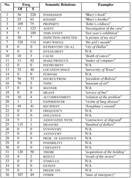
Table 1 shows the distribution of the semantic rela-tions in the annotated corpus.

In the case of of-genitives, there were 19 relations found from the total of 35 relations considered. The most frequently occurring relations were POSSES

-SION, KINSHIP, PROPERTY, PART-WHOLE, LOCA -TION,SOURCE,THEME, andMEASURE.

There were other relations (107 for of-genitives) that do not belong to the predefined list of 35 rela-tions, such as “state of emergency”. These examples were clustered in different undefined subsets based

No. Freq. Semantic Relations Examples

Of S

1 36 220 POSSESSION “Mary’s book” 2 25 61 KINSHIP “Mary’s brother” 3 109 75 PROPERTY “John’s coldness” 4 11 123 AGENT “investigation of the crew” 5 5 109 TIME-EVENT “last year’s exhibition” 6 30 7 DEPICTION-DEPICTED “a picture of my nice” 7 328 114 PART-WHOLE “the girl’s mouth” 8 0 0 HYPERNYMY(IS-A) “city of Dallas” 9 0 0 ENTAILMENT N/A 10 10 3 CAUSE “death of cancer” 11 11 62 MAKE/PRODUCE “maker of computer” 12 0 0 INSTRUMENT N/A

13 32 46 LOCATION/SPACE “university of Texas” 14 0 0 PURPOSE N/A

15 56 33 SOURCE/FROM “president of Bolivia” 16 70 5 TOPIC “museum of art”

17 0 0 MANNER N/A

18 0 0 MEANS “service of bus” 19 10 4 ACCOMPANIMENT “solution of the problem” 20 1 2 EXPERIENCER “victim of lung disease” 21 49 41 RECIPIENT “Josephine’s reward” 22 0 0 FREQUENCY N/A

23 0 0 INFLUENCE N/A

24 5 2 ASSOCIATED WITH “contractors of shipyard” 25 115 1 MEASURE “hundred of dollars” 26 0 0 SYNONYMY N/A

27 0 0 ANTONYMY N/A 28 0 0 PROB.OF EXISTENCE N/A 29 0 0 POSSIBILITY N/A 30 0 0 CERTAINTY N/A

31 120 50 THEME “acquisition of the holding” 32 8 2 RESULT “result of the review” 33 0 0 STIMULUS N/A

34 0 0 EXTENT N/A

35 0 0 PREDICATE N/A

36 107 49 OTHER “state of emergency”

Table 1: The distribution of the semantic relations in the annotated corpus of 20,000 sentences.

on their semantics. The largest subsets did not cover more than 3% of the OTHER set of examples. This observation shows that the set of 35 semantic rela-tions from Table 1 is representative for genitives.

Table 1 also shows the semantic preferences of each genitive form. For example, POSSESSION,

KINSHIP, and some kinds ofPART-WHOLErelations are most of the time encoded by the s-genitive, while some specificPART-WHOLErelations, such as “dress

of silk” and “array of flowers”, cannot be encoded

but only by the of-genitive. This simple analysis leads to the important conclusion that the two con-structions must be treated separately as their seman-tic content is different. This observation is also con-sistent with other recent work in linguistics on the grammatical variation of the English genitives (Ste-fanowitsch, 2001).

3 The Model

3.1 Problem Formulation

semantics of the noun phrases participating in geni-tives as well as the surrounding context.

Semantic classification of syntactic patterns in general can be formulated as a learning problem. This is a multi-class classification problem since the output can be one of the semantic relations in the set. We cast this as a supervised learning problem where input/ output pairs are available as training data.

An important first step is to map the characteris-tics of each genitive construction into a feature vec-tor. Let’s define withxi the feature vector of an

in-stance iand letX be the space of all instances; i.e.

xi ∈X. The multi-class classification is performed

by a function that maps the feature spaceX into a semantic spaceS

F : X → S, whereSis the set of semantic rela-tions from Table 1, i.e.rk∈S.

LetT be the training set of examples or instances

T = (x1r1,x2r2, ...,xnrn)⊆(X×S)nwherenis

the number of examplesxeach accompanied by its

semantic relation labelr. The problem is to decide which semantic relationrto assign to a new, unseen example xn+1. In order to classify a given set of

examples (members ofX), one needs some kind of measure of the similarity (or the difference) between any two given members ofX.

3.2 Feature Space

An essential aspect of our approach below is the word sense disambiguation (WSD) of the noun. Us-ing a state-of-the-art open-text WSD system with 70% accuracy for nouns (Novischi et al., 2004), each word is mapped into its corresponding WordNet 2.0 sense. The disambiguation process takes into ac-count surrounding words, and it is through this pro-cess that context gets to play a role in labeling the genitives’ semantics.

So far, we have identified and experimented with the following NP features:

1. Semantic class of head noun specifies the Word-Net sense (synset) of the head noun and implic-itly points to all its hypernyms. It is extracted au-tomatically via a word sense disambiguation mod-ule. The genitive semantics is influenced heavily by the meaning of the noun constituents. For exam-ple: “child’s mother” is a KINSHIP relation where as “child’s toy” is aPOSSESSIONrelation.

2. Semantic class of modifier noun specifies the

WordNet synset of the modifier noun. The follow-ing examples show that the semantic of a genitive is also influenced by the semantic of the modifier noun; “Mary’s apartment” is a POSSESSION rela-tion, and “apartment of New York” is a LOCATION

relation.

The positive and negative genitive examples of the training corpus are pairs of concepts of the format:

<modifier semclass#WNsense; head semclass#WNsense; target>,

wheretargetis a set of at least one of the 36

se-mantic relations. Themodifier semclassand

head semclassconcepts are WordNet semantic classes tagged with their corresponding WordNet senses.

3.3 Semantic Scattering Learning Model

For every pair of<modifier - head>noun genitives, let us define withf_imandf_jhthe WordNet 2.0 senses of the modifier and head respectively. For conve-nience we replace the tuple< fm

i , fjh > withfij.

The Semantic Scattering Model is based on the fol-lowing observations:

Observation 1.fm

i andfjhcan be regarded as nodes

on some paths that link the senses of the most spe-cific noun concepts with the top of the noun hierar-chies.

Observation 2. The closer the pair of noun senses

fijis to the bottom of noun hierarchies the fewer the

semantic relations associated with it; the more gen-eralfijis the more semantic relations.

The probability of a semantic relation r given fea-ture pairfij

P(r|fij) =

n(r, fij) n(fij)

, (1)

is defined as the ratio between the number of occur-rences of a relation r in the presence of feature pair

fij over the number of occurrences of feature pair fijin the corpus. The most probable relationˆris

ˆ

r=argmaxr∈RP(r|fij) (2)

From the training corpus, one can measure the quan-titiesn(r, fij)andn(fij). Depending on the level of

abstraction offijtwo cases are possible:

Case 1. The feature pairfijis specific enough such

P(r|fij) = 1 and0for all the other semantic

rela-tions.

Case 2. The feature pairfijis general enough such

that there are at least two semantic relations for which P(r|fij) 6= 0. In this case equation (2) is

used to find the most appropriateˆr.

Definition. A boundaryG∗

in the WordNet noun hi-erarchies is a set of synset pairs such that :

a) for any feature pair on the boundary, denoted f_ijG∗ ∈ G∗

, f_ijG∗ maps uniquely into only one rela-tionr, and

b) for anyf_iju f_ijG∗,f_iju maps into more than one relationr, and

c) for any fl ij ≺ fG

∗

ij , fijl maps uniquely into a

se-mantic relationr. Here relationsand≺mean “se-mantically more general” and “se“se-mantically more specific” respectively. This is illustrated in Figure 1.

Observation 3. We have noticed that there are more

concept pairs under the boundaryG∗

than above, i.e.

| {f_ijl} || {f_iju} |.

f_ij

G1

G2

G3

G* G4

f

ij l

fu_ij

G* f

ij G*

(b) (a)

Figure 1: (a) Conceptual view of the noun hierar-chies separated by the boundary G∗

; (b) Boundary

G∗ _{is found through an iterative process called}

“se-mantic scattering”.

3.4 Boundary Detection Algorithm

An approximation to boundary G∗ _{is found using}

the training set through an iterative process called

semantic scattering. We start with the most general

boundary corresponding to the nine noun WordNet hierarchies and then specialize it based on the train-ing data until a good approximation is reached.

Step 1. Create an initial boundary

The initial boundary denoted G1 is formed

from combinations of the nine WordNet hierar-chies: abstraction#6, act#2, entity#1, event#1, group#1, possession#2, phenomenon#1, psycholog-ical feature#1, state#4. To each training exam-ple a corresponding feature fij =< fim, fjh >

is first determined, after which is replaced with the most general corresponding feature consisting of top WordNet hierarchy concepts denoted with

f_ij1. For instance, to the example “apartment of the

woman” it corresponds the general feature entity#1-entity#1 and POSSESSION relation, to “husband of

the woman” it corresponds entity#1-entity#1 and

KINSHIP relation, and to “hand of the woman” it corresponds entity#1-entity#1 andPART-WHOLE

re-lation. At this high levelG1, to each feature pairf_ij1

it corresponds a number of semantic relations. For each feature, one can determine the most probable relation using equation (2). For instance, to feature

entity#1-entity#1 there correspond 13 relations and

the most probable one is the PART-WHOLE relation

as indicated by Table 2.

Step 2. Specialize the boundary 2.1 Constructing a lower boundary

This step consists of specializing the semantic classes of the ambiguous features. A feature f_ijk

on boundary Gk is ambiguous if it corresponds to more then one relation and its most relevant rela-tion has a condirela-tional probability less then 0.9. To eliminate non-important specializations, we special-ize only the ambiguous classes that occurs in more than 1% of the training examples.

The specialization procedure consists of first identifying features fk

ij to which correspond more

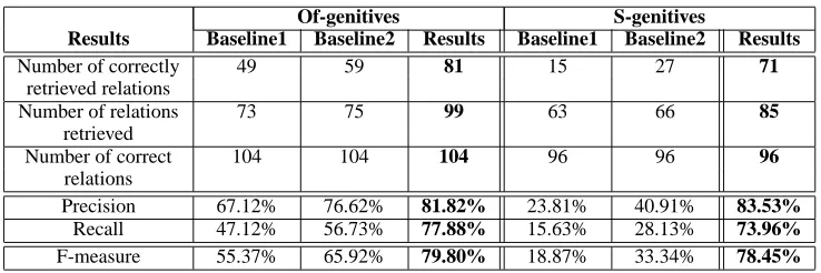
than one semantic relation, then replace these tures with their hyponyms synsets. Thus one fea-ture breaks into several new specialized feafea-tures. The net effect is that the semantic relations that were attached to f_ijk will be “scattered” across the new specialized features. This process continues till each feature will have only one semantic relation at-tached. Each iteration creates a new boundary, as shown in Figure 1. Table 3 shows statistics of se-mantic features f_ijk for each level of specialization

Gk. Note the average number of relations per fea-ture decreasing asymptotically to1askincreases.

R 1 2 3 6 7 11 13 15 16 19 21 24 25 Others

P(r|entity−entity) 0.048 0.120 0.006 0.032 0.430 0.016 0.035 0.285 0.012 0.004 0.010 0.001 0.001 0

Table 2: Sample row from the conditional probability table where the feature pair is entity-entity. The numbers in the top row identify the semantic relations (as in Table 1).

Of-genitives S-genitives

Boundary G1 G2 G3 G1 G2 G3

Number of modifier 9 31 74 9 37 91

features

Number head 9 34 66 9 24 36

features

No. of feature pairs 63 out of 81 216 out of 1054 314 out of 4884 41 of 81 157 out of 888 247 out of 3276

Number of features 26 153 281 14 99 200

with only one relation

Average number of 3 1.46 1.14 3.59 1.78 1.36

relations per feature

Table 3: Statistics for the semantic class features by level of specialization.

The new boundary is more specific then the previ-ous boundary and it is closer to the ideal boundary. However, we do not know how well it behaves on unseen examples and we are looking for a boundary that classifies with a high accuracy the unseen exam-ples. We test the boundary on unseen examexam-ples. For that we used 10% of the annotated examples (differ-ent from the 10% of the examples used for testing) and compute the accuracy (f-measure) of the new boundary on them.

If the accuracy is larger than the previous bound-ary’s accuracy, we are converging toward the best approximation of the boundary and thus we should repeat Step 2 for the new boundary.

If the accuracy is lower than the previous bound-ary’s accuracy, the new boundary is too specific and the previous boundary is a better approximation of the ideal boundary.

For the automatic detection of the semantic re-lations encoded by genitives, the boundary con-structed by the Semantic Scattering model is more apppropriate than a “tree cut”, like the ones used for verb disambiguation (McCarthy, 1997) (Li and Abe, 1998) and constructed using the Minimum Descrip-tion Length model (Rissanen, 1978). The develope-ment of a ”tree cut” model for the detection of the semantic relations encoded by genitives involves the construction of a different ”tree cut” for each head noun and threfore the usage of these cuts is restricted to those head nouns. On the other hand, Semantic Scattering constructs only one boundary that, unlike

the ”tree cut” model, is general enough to classify any genitive construction, including the ones with constituents unseen during training.

4 Semantic Relations Classification

Algorithm

The ideal boundary G∗ _{is used for classifying the}

semantic relations encoded by genitives. The algo-rithm consists of:

Step 1. Process the sentence. Perform Word Sense

Disambiguation and syntactic parsing of the sen-tence containing the genitive.

Step 2. Identify the head and modifier noun con-cepts.

Step 3. Identify the feature pair. Using the results

from WSD and WordNet noun hierarchies, map the head and modifier concepts into the corresponding classes from the boundary and identify a feature pair

fijthat has the closest euclidean distance to the two

classes.

Step 4. Find the semantic relation. Using the feature fij, determine the semantic relation that corresponds

to that feature on the boundary. If there is no such relation, mark it asOTHER.

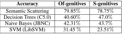
5 Results

For testing, we considered 20% of the annotated ex-amples. We used half of the examples for detecting the boundaryG∗

and half for testing the system.

G∗

Boundary Detection

Of-genitives S-genitives

Results Baseline1 Baseline2 Results Baseline1 Baseline2 Results

Number of correctly 49 59 81 15 27 71

retrieved relations

Number of relations 73 75 99 63 66 85

retrieved

Number of correct 104 104 104 96 96 96

relations

Precision 67.12% 76.62% 81.82% 23.81% 40.91% 83.53% Recall 47.12% 56.73% 77.88% 15.63% 28.13% 73.96% F-measure 55.37% 65.92% 79.80% 18.87% 33.34% 78.45%

Table 4: Overall results for the semantic interpretation of genitives

specializations on the WordNet IS-A noun hierar-chies in order to eliminate the ambiguities of the training examples. BoundaryG1 corresponds to the semantic classes of the nine WordNet noun hier-archies and boundaries G2 and G3 to their subse-quent immediate hyponyms. For both s-genitives and of-genitives, boundary G2 was more accurate then boundary G1 and therefore we repeated Step 2. However, boundary G3 was less accurate then boundary G2 and thus boundary G2 is the best ap-proximation of the ideal boundary.

Semantic Relations Classification

Table 4 shows the results obtained when classify-ing the 36 relations (the 36th relation beclassify-ingOTHER) for of-genitives and s-genitives. The results are pre-sented for the Semantic Scattering system that uses

G2as the best approximation of theG∗_{together with}

two baselines. Baseline1 system obtained the re-sults without any word sense disambiguation (WSD) feature, i.e. using only the default sense number 1 for the concept pairs, and without any specializa-tion. Baseline2 system applied two iterations of the boundary detection algorithm but without any word sense disambiguation.

Overall, the Semantic Scattering System achieves an 81.82% precision and 77.88% recall for of-genitives and an 83.53% precision and 73.96% re-call for s-genitives.

Both the WSD and the specialization are impor-tant for our system as indicated by the Baseline systems performance. The impact of specializa-tion on the f-measure (Baseline2 minus Baseline1) is 10.55% for of-genitives and 14.47% for s-genitives, while the impact of WSD (final result minus Base-line2) is 14% for of-genitives and 45.11% for s-genitives.

Error Analysis

An important way of improving the performance of a system is to perform a detailed error analysis of the results. We have analyzed the various error sources encountered in our experiments and summarized the results in Table 5.

Error Type Of-genitives S-genitives %Error %Error Missing feature 28.57 29.17 General semantic classes 28.57 20.83

WSD System 19.05 29.17

Reversed order of constituents 14.29 12.5 Named Entity Recognizer 4.76 8.33 Missing WordNet sense 4.76 0

Table 5: The error types encountered on the testing corpus.

6 Comparison with other Models

To evaluate our model, we have conducted ex-periments with other frequently used machine learning models, on the same dataset, using the

same features. Table 6 shows a comparison

between the results obtained with the Semantic Scattering algorithm and the decision trees (C5.0,

http://www.rulequest.com/see5-info.html), the

naive Bayes model (jBNC, Bayesian Network Classifier Toolbox, http://jbnc.sourceforge.net), and Support Vector Machine (libSVM,

Chih-Chung Chang and Chih-Jen Lin. 2004.

three models normally work better with a larger set of features.

Accuracy Of-genitives S-genitives Semantic Scattering 79.85% 78.75%

Decision Trees (C5.0) 40.60% 47.0%

Naive Bayes (JBNC) 42.31% 43.7%

SVM (LibSVM) 31.45% 23.51%

Table 6: Accuracy performance of four learning models on the same testing corpus.

7 Discussion and Conclusions

The classification of genitives is an example of a learning problem where a tailored model outper-forms other generally applicable models.

This paper presents a model for the semantic clas-sification of genitives. A set of 35 semantic relations was identified, and we provided statistical evidence that when it comes to genitives, some relations are more frequent than others, while some are absent. The model relies on the semantic classes of noun constituents. The algorithm was trained and tested on 20,000 sentences containing 2,249 of-genitives and 1006 s-genitives and achieved an average preci-sion of 82%, a recall of 76%, and an f-measure of 79%. For comparison, we ran a C5.0 learning sys-tem on the same corpus and obtained 40.60% accu-racy for of-genitives and 47% for s-genitives. A sim-ilar experiment with a Naive Bayes learning system led to 42.31% accuracy for of-genitives and 43.7% for s-genitives. The performance with a Support Vector Machines learner was the worst, achieving only a 31.45% accuracy for of-genitives and 23.51% accuracy for s-genitives. We have also identified the sources of errors which when addressed may bring further improvements.

References

Barker, Chris. 1995. Possessive Descriptions. CSLI Publications, Standford, CA.

Berland, Matthew and Eugene Charniak. 1999. Finding parts in very large. In Proceeding of ACL 1999.

Fellbaum, Christiane. 1998. WordNet - An Electronic

Lexical Databases. Cambridge MA: MIT Press.

Girju, Roxana, Adriana Badulescu, and Dan Moldovan. 2003. Learning semantic constraints for the automatic discovery of part-whole relations. In Proceedings of

the HLT-NAACL 2003.

Gildea, Daniel and Daniel Jurafsky. 2002. Automatic Labeling of Semantic Roles. Computational

Linguis-tics, 28(3):277-295.

Hearst, Marti. 1998. Automated Discovery of Word-Net relations. In An Electronic Lexical Database and

Some of its Applications. MIT Press, Cambridge MA.

Lapata, Maria. 2000. Automatic Interpretation of Nomi-nalizations. In Proceedings of AAAI 2000, 716-721.

Li, Hang and Naoki Abe. 1998. Generalizing case frames using a thesaurus and the mdl principle.

Com-putational Linguistics, 24(2):217–224.

McCarthy, Diana. 1997. Word sense disambiguation for acquisition of selectional preferences. In Proceedings

of the ACL/EACL 97.

Moldovan, Dan, Adriana Badulescu, Marta Tatu, Daniel Antohe, and Roxana Girju. 2004. Models for the Se-mantic Classification of Noun Phrases. In

Proceed-ings of the HLT-NAACL 2004, Computational Lexical Semantics Workshop.

Nikiforidou, Kiki. 1991. The meanings of the genitive: A case study in the semantic structure and semantic change. Cognitive Linguistics, 2:149–205.

Novischi, Adrian, Dan Moldovan, Paul Parker, Adriana Badulescu, and Bob Hauser. 2004. LCC’s WSD

sys-tems for Senseval 3. In Proceedings of Senseval 3.

Rissanen, Jorma. 1978. Modeling by shortest data de-scription. Automatic, 14.

Rosario, Barbara and Marti Hearst. 2001. Classify-ing the Semantic Relations in Noun Compounds via a Domain-Specific Lexical Hierarchy. In Proceeding

of EMNLP 2001.

Siegel, S. and N.J. Castellan. 1988. Non Paramet-ric Statistics for the behavioral sciences. New York:

McGraw-Hill.

Stefanowitsch, Anatol. 2001. Constructional semantics as a limit to grammatical alternation: Two genitives of English. Determinants of Grammatical Variation in

English.

Taylor, John. 1996. Possessives in English. An ex-ploration in cognitive grammar. Oxford, Clarendon

Press.

Vikner, Carl and Per Anker Jensen. 1999. A semantic