L Inference for shape parameter estimation

(1)

L

₂

Inference for Shape Parameter Estimation

by

Claudia L. Arellano Vidal, MSc

Dissertation

Presented to the University of Dublin, Trinity College

in fulfillment of the requirements for the Degree of

Doctor of Philosophy

University of Dublin, Trinity College

(2)

(3)

(4)

(5)

Declaration

I, the undersigned, declare that this work has not previously been submitted as an

exercise for a degree at this, or any other University, and that unless otherwise stated, is

my own work.

Claudia L. Arellano Vidal

(6)

(7)

Permission to Lend and/or Copy

I, the undersigned, agree that Trinity College Library may lend or copy this thesis

upon request.

Claudia L. Arellano Vidal

(8)

(9)

Abstract

In this thesis, we propose a method to robustly estimate the parameters that controls the mapping of a shape (model shape) onto another (target shape). The shapes of interest are

contours in the 2D space, surfaces in the 3D space and point clouds (either in 2D and 3D spaces). We propose to model the shapes using Gaussian Mixture Models (GMMs)

and estimate the transformation parameters by minimising a cost function based on the Euclidean (L2) distance between the target and model GMMs. This strategy allows us to

avoid the need for the computation of one to one point correspondences that are required by state of the art approaches making them sensitive to both outliers and the choice of

the starting guess in the algorithm used for optimisation.

Shapes are well represented by GMMs when careful consideration is given to the

design of the covariance matrices. Compared to isotropic covariance matrices, we show how shape matching withL2can be made more robust and accurate by using well chosen

non isotropic ones. Our framework offers a novel extension toL2based cost functions by

allowing prior information about the parameters to be included. Our approach is therefore

fully Bayesian.

This Bayesian-L2 framework is tested successfully for estimating the affine

trans-formation between data sets, for fitting morphable models and fitting ellipses. Finally we show how to extend this framework to shapes defined in higher dimensional feature

(10)

(11)

Acknowledgments

This thesis would not have been possible without the help, support and patience of my principal supervisor Dr Rozenn Dahyot. She used to say that she was not my supervisor

but just an advisor instead. But the truth is that she was my super-advisor. I really appreciate all the good advices, the encouragement she gave me along this process and

above all her friendship. I would also like to express my gratitude to my co-supervisor, Professor Kurshid Ahmad for all his useful advice not only about the thesis but also

about life in general. I would like to acknowledge to Trinity College Dublin and the Government of Chile for the financial support. Thanks to all GV2 group and in particular

to Jonathan, Stefan, Mirko, Fintan and Ludovic for all their help. Special thanks to Ziggy for proofreading my thesis and most of my papers.

I had a wonderful time in Ireland while I was writing my doctoral thesis and I owe that to all the wonderful people I had around. I am very greatful for the company and

friendship of Atul, Kerstin, Katja and Ziggy. Thank you guys for all the movie nights, the long chats, the laugh and the good times. Special thanks to Soraya, Eonmi, Christina

and Venkat for being not only good friends but also my family while living in Dublin. My gratitude to my boyfriend Joe for all his support and patience.

Finally, I wish to thank my parents and my sister for their love and encouragement. Without them I would never have had so many opportunities.

C

LAUDIA

L. A

RELLANO

V

IDAL

University of Dublin, Trinity College

(12)

(13)

List of Tables

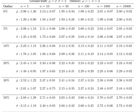
3.1 Average estimates of the mean and standard deviation with their confi-dence intervals (100 runs) with varying proportions of outliers and sam-ple size. . . 37

3.2 The global minimum depends on the selected fixed bandwidthσ. . . 37

5.1 Numerical assessment of the experiments displayed in Figure 5.1a. In this case we set both algorithms to use the same parameters. . . 60

5.2 Numerical assessment of the experiments displayed in Figure 5.1b. In this case we include the annealing strategy for improving convergence of the Mean Shift Algorithm. . . 61

5.3 Numerical assessment of the experiments displayed in Figure 5.1c. This case is similar to the previous one (case b) where the annealing strategy is included in the Mean Shift Algorithm. . . 61

5.4 Rate of convergence towards the ground truth when considering an error of±10 . . . 66

5.5 Run-time performance of the algorithm measured as the time it takes the algorithm to converge (in seconds). . . 67

5.6 Computational complexity of the algorithm. . . 67

5.7 A comparison of the convergence of isotropic versus non-isotropic mod-ellings for drastically sub-sampled data sets. . . 70

5.8 The rate of convergence towards the ground truth when considering error of 5%. We evaluate the cases where: no changes are made in the data (original), data is perturbed with noise (levels: 0.01 and 0.03), data is perturbed with outliers, and occluded data. In all cases 100 experiments were run and the number of successes are reported in the table. . . 72

5.9 The rate of convergence towards the ground truth when considering an error of 10% and 5%. The bandwidth for this experiment was set to

(18)

5.10 Paired difference test: The table shows the value for the mean (d¯), stan-dard deviation (σd), number of samples (no) and the t-value calculated as t= _σd¯−0

d/

√

n . . . 81

6.1 Comparison of the convergence rate between isotropic and non-isotropic modelling . . . 87 6.2 Malahanobis distancedi,j between the estimated parameters of faces F1

to F6 (Figure 6.13). . . 95

(19)

List of Figures

1.1 Computer generated image of a room full of chairs [1] . . . 1 1.3 Example of the parameter estimation problems to be considered in this

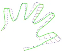
thesis. Figure a) shows two shapes (hand). The two shapes are aligned to each other and displayed in Figure b). Figure c) shows the fitting process performed where one of shape is deformed in order to represent the second shape as close as possible. . . 2 1.2 Examples of three shapes. Figure a) shows a parametric curve (ellipse).

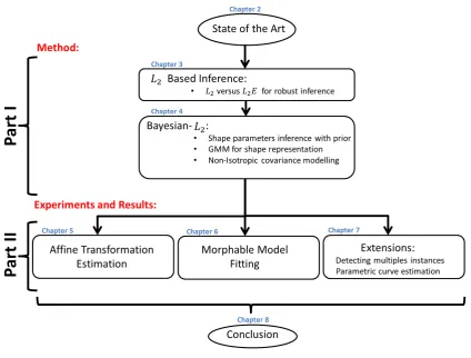
Figure b) shows a 2D contour model of a hand and Figure c) shows a surface representation of a human face (3D mesh). . . 2 1.4 Point to point correspondence between shapes . . . 3 1.5 Thesis outline. . . 6

2.1 Structural shape representation. The shape is broken down in segments that are represented individually. In a) we reprinted a horse shape that has been represented usingcurvatureandorientationreported in [2]. The structural description of a chromosome shape described in [2] is shown in b) and the primitives used are shown in c). . . 9 2.2 Global shape description. Figure in a) represents a shape contour that

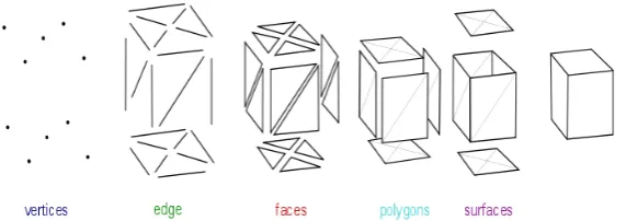
can be defined using the one dimensional function shown in b)x(t) = cos(2t). The representation of the character M in c) can be described using its edge image d). . . 10 2.3 Point Cloud description by sampling the edge image. . . 11 2.4 Point Cloud description by sampling the edge image. . . 11 2.5 3D mesh representation using different resolutions (increasing the

num-ber of faces) [3]. . . 11 2.6 Statistical inference using parametric modelling. In a) a set of

(20)

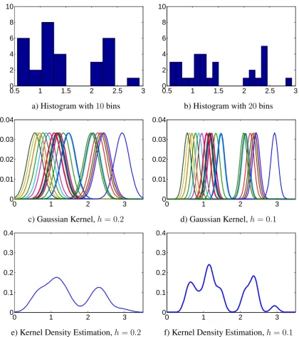
2.7 This figure shows the two approaches in non-parametric modelling: His-tograms and kernel density estimation. We model the density function given a set of n = 30 observations. In the top row we present the his-togram of the data set when using a)10and b)20bins. In the middle row the same data set is represented using a Gaussian kernel for each point in the data set and using a bandwidth ofh= 0.2andh= 0.1(Figures c and d respectively). Finally the density estimation using the kernels in c) and d) are presented in e) and f) respectively. . . 14 2.8 Scheme of SOM [4] . . . 17 2.9 Example of Self Organizing map for diferents iterations. The dots are

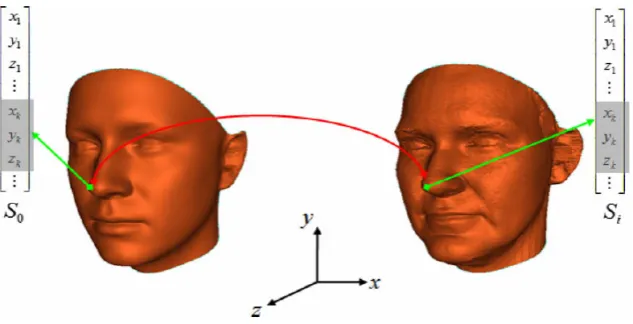
the set of observations. The grid is a set of connected nodes that are automatically organised to represent the observations [4] . . . 18 2.10 Point to point correspondence between data sets. [5] . . . 19 2.11 The shape correspondence concept of the 3D Morphable Model: The

figure illustrates how vertices are indexed in the parametrized domain. For instance, according to Levine et al. [6], the tip of the nose will be assigned in the same position (k) in the vector shape si in every scan,

even though the coordinate x, y and z that represent its position will change among individuals. . . 24

3.1 Example: a) Normal distributiong(x|Θ = (µ = 2, σ = 2)). Figure b) shows a set of observations sampled fromg (black dots) and Figure c) shows the empirical distributionfˆassociated with the observations. The empirical distribution is represented by a delta Dirac function centred in each observation. . . 33 3.2 Results obtained when running 100 experiments for samples sizes of

5,10,50,100,1000and10000reported on the abscissa. The figure shows the average error between the ground truth and the estimates with a95% confidence interval for the mean in a) and standard deviation in b). In both cases the error decreased when increasing the number of samplesnf. 34

3.3 The figure shows a set of samples taken from the true density function

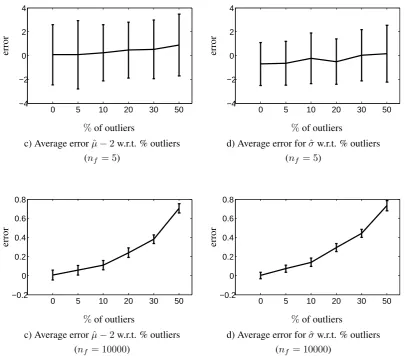
g(x|Θ = (µ = 2, σ = 2)), and a few outliers drawn from a different density function (in red dash line). . . 35 3.4 Average error (between ground truth and estimates) with95%confidence

intervals with sample sizenf = 5(top row) andnf = 10000(bottom row). 36

3.5 Estimates (100 experiments) with meanµˆ reported in absissa andσˆ on the y-axis (0% outliers). The ground truth(µ, σ) = (2,2)is plotted in black, estimates withnf = 100 (blue) and estimates with nf = 10000

(21)

3.6 Estimates (100 experiments) for nf = 10000 with mean µˆ reported in

abscissa andσˆ on the y-axis. The ground truth(µ, σ) = (2,2)is plotted in black. The estimates without outliers are shown in red, the estimated with20% of outliers are shown in purple and the green one correspond to the estimated using50%of outliers. . . 38

3.7 Cost function (L2E(µ)) for a sample sizenf = 5with two outliers. The

red line corresponds toσ= 1, blue dashed (σ= 1.5), green dots (σ= 3) and black dash-dot (σ = 5). The figure shows the impact of the band-width on the estimation ofµusing theL2E approximation. . . 39

4.1 Modelling when using isotropic covariance matrices. . . 46

4.2 Effects of choosing a) proportional weight for the Gaussians instead of b) uniform weights. The ridge in a) has a similar value along the shape while in b) the ridge changes value along the shape. . . 47

4.3 Scheme of the principal directions of the covariance matrix extracted from a given 3D mesh . . . 48

4.4 Reduction of the number of Gaussians in the mixture to represent the shape. 50

4.5 Similarity between shapes (Euclidean distance) when modelling the GM using non-isotropic covariance matrices and different numbers of Gaus-sians in the mixture. . . 51

4.7 Example of a portion of the mesh of a face when described using a differ-ent number of vertices. As more vertices are used (left) a more accurate representation is produced. . . 51

4.6 Density functions computed from the hand model when using non-isotropic Gaussians (withn = 71,n= 56,n= 39andn= 31kernels from top to bottom respectively). . . 52

4.8 Example of the meshing process using SOM. Figure a) shows the original 3D point cloud (blue dots) and the starting position of the mesh (red). Figures b) and c) show the final solution for different numbers of vertices (100 and 400, respectively). . . 53

(22)

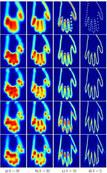
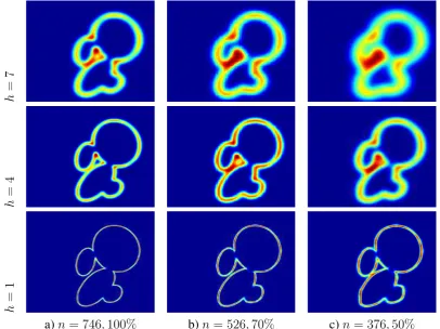
4.10 2D view of the density function computed for Figure 4.11a. In the first column we show the density functions when using all data (764 points) for bandwidths of 7, 4 and 1 respectively. The second column shows the density functions of the observations with a resolution of70%and in the last column with resolution of50%. The number of Gaussians used to define the density functions are 526 and 372 respectively. In the three cases, the rows shows the 2D views when different bandwidths are used. At the toph= 7, in the middle rowh = 4and in the bottom rowh= 1. . 54 4.11 The set of observations are extracted from the image a). We use the edge

map and the gradient of the image to compute the position and curvature of the points of interest. In b) we show the map of the normal vector associated to the edge map. In c) we show the computed observation

{(ui, ψi)}i=1···,n ∈R3. . . 56

5.1 2D data sets: alignment obtained when testing the 2D data sets Fish, Contour and a Chinese Character: Reference point set (blue circles), ob-servation (red asterisk) and estimated solution (green cross). The top row of the figure shows results obtained using Jian and Vermuri’s algorithm while in the bottom row we show the convergence obtained using our proposed MS algorithm. . . 61 5.2 Examples of the experiment performed for an angle of rotation ofφGT =

30o_{. Results are displayed for our proposed algorithm, KC registration}

and ICP registration. . . 63 5.3 Convergence rate (%) of the estimated solution (y-axis) when perturbing

the data with different noise levels (x-axis) using our proposed algorithm (red line) and when using the Kernel Correlation algorithm (blue dot-dash line). In a) we show the results for a rotation angle ofφGT = 20o

and in b)φGT = 30o . . . 64

5.4 Error mean with95%of confidence of the estimated rotation when data is perturbed using different levels of noise (from 0 to 0.2). In a) we show the target angle or rotation isφGT = 20oand in b)φGT = 30o . . . 64

5.5 Examples when both sets are rotated by20o. . . 65 5.6 Examples when both sets are rotated by90o_{. . . 65}

(23)

5.8 Example of a set of observations a) and model of the hand b) used for estimating the rigid transformation when modelling GMM using non-isotropic covariance matrices. In c) we show a sub-sampled version of the hand model. . . 68

5.9 Cost function computed when both GMMs are modelled using isotropic covariance matrices (blue dash line) and when one of them is modelled using non-isotropic modelling (red line). . . 69

5.10 An example of results obtained when sub-sampling the data sets and when using isotropic (green dash line) and non-isotropic modelling (red line). The blue dots correspond to the full observation. . . 70

5.11 Examples of the data set used for testing . . . 71

5.12 Examples of the results obtained when testing our algorithm under dif-ferent conditions. . . 73

5.13 Experiment setup. The object to be scanned is placed as close as possible to the Kinect sensor (approximately 50 cm). The object (here a head) is rotated in order to capture different points of view. . . 74

5.14 Results obtained when aligning different views captured using the Kinect sensor. The noise is reduced as the number of viewsnmerged increase. A laser scanner acquisition is also shown for visual comparison purposes . 75

5.15 Kinect scan alignment for a face. The top row shows a sequence of im-ages captured from different points of view. Bottom row: Mesh created from a) a single acquisition, b) multiples views and c) face captured using a laser scanner. . . 75

5.16 a) the picture of the object (Duck) and d) laser scan respectively (ground truth). In b) the reconstruction with one acquisition using the Kinect sensor and e) its error w.r.t. the laser scan has an average of 2.25mm. When merging 15 views together c) the average error f) is reduced to 1.54mm. Details of the Gnome face the average error of the reconstructed shape when four images are merged is1.7mm. . . 76

5.17 Two scans displayed from different viewpoints . . . 77

(24)

5.19 A set of scans aligned together. The figure on the left shows a set of 6 consecutive scans. The middle figure shows the results after estimating the transformation parameters between the scans. The same result from another point of view is displayed in the right figure . . . 79

5.20 The distance between the shape when aligned using the proposed method (blue line) and when aligned using the ground truth (red line). Results obtained when modelling the density function using isotropic bandwidth

h= 7,14,21and35. . . 79

5.21 Details of the alignment between buildings. a) using our proposed algo-rithm for aligning the scans and b) using ground truth. . . 81

6.1 Overview of the shape estimation process using a shape model as prior information. The observation as a point cloud {ui}i=1,···,n in b) is

ob-tained after preprocessing the image a) captured by a 2D camera sensor. The parameter estimation is then divided into two steps: c) shape align-mentΘ = [s,R,t]and d) shape fittingΘ = [α]. . . 84

6.2 Results obtained when using synthetic hands generated from the model a) and when adding random noise b). Figures c) and d) show the estimated shape when the prior information is not considered in the algorithm. In all figures: observations (blue dots), initial guess (green dash) and estimated solution (red line). Setting: hmax = 50,hmin = 5. . . 85

6.3 Hand model fitting to a point cloud obtained from 2D images. Column a) and b) show the colour image and edge map used for the experiments. In column c) the estimated hands (red dash) and in d) the solution when the prior is not used in the algorithm. For the two experiments we com-pute the Euclidean distanced between the model and the observations. When using the prior information the algorithm minimises the Euclidean distance better (results in c) than when the prior is not used d). . . 86

6.4 Examples of observations when randomly sub-sampling the original data set. . . 87

(25)

6.6 Examples of results obtained when reducing the number of Gaussians for the shape model (ng). Top row shows results of the estimation when

using non-isotropic covariance matrices. The bottom row shows results when using isotropic covariance matrices. In all examples, the red line corresponds to the estimate while the blue dots to the observations. . . 89 6.7 Fitting synthetic faces: target face (observations, top row), random

start-ing guess for initialisstart-ing the algorithm (middle row) and estimated face with our algorithm (bottom row). . . 90 6.8 Surface error computed between the target face and our reconstruction. . . 90 6.9 Preprocessing for generating the points cloud of the face (target): depth

map (a) as captured by the RGB-D sensor, selection of the scene (b) in close range (between0.5mand1.2mfrom the sensor), extracted face and skin region (c). . . 91 6.10 Shape alignment: different views of the point clouds (model (grey) and

observations (red)) after alignment (top row). Same point clouds dis-played before alignment (bottom row). . . 92 6.11 Histogram of the errors between the observations to the average shape:

before alignment (blue) and after (red). The sum of the absolute error is 6.3456×106 _{(after alignment) compared with} ₁_.₇₀₅₄_×₁₀7 _(before

alignment). . . 93 6.12 Average shape used as initial guess. . . 93 6.13 Estimated reconstructed faces (labelled F1 (top), to F6 (bottom)) from 3

viewpoints shown with the colour image captured with the Kinect (left). . 94 6.14 At the top, profile view of F5: laser scan (left), reconstruction (middle)

and Kinect point cloud (right). At the bottom, frontal view of F5: recon-struction (left) and laser scan (right). . . 95 6.15 Histograms of the errors between the observations and the reconstructed

face (red line) and the observations and the average shape of the model (blue dash) for F1 (left) and F2 (right). . . 95 6.16 Percentage of observations below a distance between 1 and 5mm

(re-ported on the absissa) for F1 (left) and F2 (right), before fitting (blue dash) and after fitting (red line). . . 96 6.17 Values of the J = 20 coordinates of parameter α normalised with the

eigenvalues computed for faces F1 to F6. . . 96

7.1 Example of detection of multiples instance (i.e coins). . . 98 7.2 Illustration of the iteration of the proposed method for detecting multiple

(26)

7.4 Example of the GMM of the ellipse computed using different bandwidths. 103

7.5 Figure shows three examples of observation used in the experiments. The ellipses were computed using the target ellipse for which the parameters are Θ = [γ, a, b, xo, yo] = [0,3,5,0,0]corrupted using Gaussian noise

with standard deviationσ2equal to0.1,0.3and0.5respectively . . . 103

7.6 Example of computing the error rate. Figure a) shows in blue the true ellipse (observation) and in red dots the estimated one. The black region in figure b) represents the area of the symmetric difference in between the two ellipses. . . 104

7.7 Mean Error obtained for the data sets perturbed with 5 different standard deviation of noise (σ from 0.1 to 0.5). In a) we compare the proposed method (green star) versus a recent robust ellipse fitting algorithm re-ported by Yu et al. [7] (blue square). In b) our proposed method (green start) is compared with two standard ellipse fitting algorithms. The red triangle represents the algorithm which cost function minimises the alge-braic distance while the blue dot is the well known Least Square method that is based on the minimisation of a geometric distance . . . 105

7.8 Figure shows a detail of the error of each method including its95% of confidence interval. . . 105

7.9 Results of the mean error compared with standard fitting ellipse methods for 5 level of noise. This experiment corresponds to the case where10% of extra points randomly distributed are added to the observation. The er-ror computed when using our proposed method (green start) is compared with two standard ellipse fitting algorithms. The red triangle represents the algorithm which cost function minimises the algebraic distance while the blue dot is the well known Least Square method that is based on the minimisation of a geometric distance [8, 9]. . . 106

7.11 Results compared two ellipses. For our method we run a trial of 50 ex-amples obtaining a mean error of 0.0133 with a standard deviation of 0.0012. When perturbed using σ = 0.1. In all the figures the red dots correspond to the observation. In a) we show the results obtained using the direct fit algorithm, in b) Least Square method and in c) our proposed method. . . 106

(27)

7.12 This Figure shows an example of the data set used for testing the algo-rithm. This data set was published by [10] and it contains 6 sets of 50 images. Each set contains a different number of occluded ellipses from 4 to 24. In the first and third row the original images are displayed while in the second and forth the observations extracted are shown as a map of normal vector corresponding to the edge points in the original image. . . . 109 7.13 Example of the results obtained when applying our proposed algorithm

for detecting multiples ellipses. On the top row the original images and at the bottom the detected ellipses (red) and the observations (blue). . . . 110 7.14 Example of the results obtained when applying our algorithm to data sets

containing 4,8,12,16,20 and 24 occluded ellipses respectively. . . 111 7.15 Testing on synthetic images containing occluded images. In Figure a)

we report the values obtained for the Recall while in b) the results for precision. Each set (from 4 to 24) was evaluated using 50 images. For comparison we report the results obtained using the approaches proposed by Chia et al.[10], Mai et al. [11], Kim et al [12] and the Hough transform based methods RHT and SHT proposed by [13] and [14] respectively. . . 112 7.16 Testing our algorithm on 50 synthetic images each containing four 4

el-lipses occluded as overlap error is varied from 0.05 to 0.55. . . 112 7.17 Examples of detecting ellipses in RGB images. . . 112

C.1 Example 1 of results obtained for noise level 1 and angle of rotation30o _{. 127}

C.5 Example 5 of results obtained for noise level 1 and angle of rotation90o . 129 C.6 Example 6 of results obtained when both sets are rotated in45o _{. . . 130}

C.7 Example 1 scaling . . . 130 C.8 Example 2 scaling . . . 131 C.9 Example 3 scaling . . . 131 C.10 Example 4 scaling . . . 131 C.11 Top: Results fors1, estimated (blue line) and ground truth (red square).

Bottom shows the results fors2. The experiments where performed using

the same data sets scaled using a normal distribution for both parameters. We run 100 experiments and all of them converge to the ground truth. . . 132 C.12 Top: Results fors1, estimated (blue line) and ground truth(red square).

(28)

C.13 Example scaling with outliers in the data set . . . 134 C.14 Example 1 scaling with outliers in the data set . . . 134 C.15 Example 2 scaling with occlusion in the data set . . . 134 C.16 Example 3 scaling with occlusion in the data set . . . 135 C.17 Top: Results for s1, estimated (blue line) and ground truth(red square).

the occluded data set which was scaled using a normal distribution for both parameters. . . 136 C.18 Example 4 scaling with noisy data set . . . 137 C.19 Example 5 scaling with noisy data set . . . 137 C.20 Example 6 scaling with noisy data set . . . 137 C.21 Example 7 scaling with noisy data set (S1) . . . 138

C.23 Example 1 Occlusion (25%) and Outliers (20%) Examples (using prior) . 138 C.24 Example 2 Occlusion (25%) and Outliers (20%) Examples (using prior) . 138 C.22 Example 8 scaling with noisy data set (S2) . . . 139

C.25 Example 3 Occlusion (25%) and Outliers (20%) Results for S1 andS2

(with prior) . . . 139 C.26 Results of the parameters estimated using our proposed method. . . 140 C.27 Estimated shapes (in red solid line) using the isotropic shape model (a)

and the non-isotropic shape model (b). The observations are shown as blue dots. . . 141 C.28 The green line correspond to the non-isotropic model and the blue dots

(29)

Chapter 1 Introduction

Human vision is a powerful perceptual system that allows us to understand the world. This process of understanding is usually based on the classification and identification of objects we can see. One of the attributes that most distinguishes an object from its surroundings is its shape. It is well known and commonly accepted that the mechanism underlying the human perception of shapes is innate. This innate human ability is so pow-erful that objects that has been rotated, scaled or even occluded can be still be recognised. A well known example is shown in Figure 1.1 where a room full of chairs is displayed. There is no difficulty for humans to recognise the chair partially hidden behind the desk or the small rotated version hanging from the ceiling.

Figure 1.1: Computer generated image of a room full of chairs [1]

(30)

a) b) c)

Figure 1.3: Example of the parameter estimation problems to be considered in this the-sis. Figure a) shows two shapes (hand). The two shapes are aligned to each other and displayed in Figure b). Figure c) shows the fitting process performed where one of shape is deformed in order to represent the second shape as close as possible.

estimating those transformation parameters between shapes in order to achieve methods for detecting and reconstructing them. In this thesis the focus will be on shapes that can be represented either using a parametric expression or by a set of points (i.e point cloud, meshes etc.). Examples of shapes are shown in Figure 1.2.

a) Ellipse b) Hand c) Face

Figure 1.2: Examples of three shapes. Figure a) shows a parametric curve (ellipse). Fig-ure b) shows a 2D contour model of a hand and FigFig-ure c) shows a surface representation of a human face (3D mesh).

1.1 Overview and motivation

Estimating the parameters of a shape is a problem that arises in different fields in com-puter vision. The problem is usually classified according to the parameters to be esti-mated, the knowledge or information about the shape and the kind of observation that is being dealt with. Two general categories related to shape parameter estimation found in the literature and that we will study areshape alignmentandshape fitting.

(31)

[image:31.595.256.364.68.156.2]

Figure 1.4: Point to point correspondence between shapes

process is commonly referred to as shape registration. Registration of shapes usually involves a second process where point correspondence between the two shapes needs to be computed (cf. Figure 1.4). The correspondence between shapes is not a trivial prob-lem and usually introduces error when estimating parameters, in particular when the two shapes are not defined using the same description.

Shape Fitting: A statistical shape model is deformed in order to fit a set of observa-tions (cf. Figure 1.3c). Many state of the art methods solving this problem require the model and the observation to be aligned. Additionally, the correspondences between the two shapes need to be established. The need for correspondences imply that the fitting algorithm depends directly on the previous step: registration. Any error in the correspon-dences is directly reflected in the parameters estimated during the fitting process. This makes fitting algorithms very sensitive, especially to outliers and noise in the data.

1.2 Current problems and scope of the present work

Shape fitting algorithms still depend on the accuracy of the correspondences. Indeed, errors in the correspondence in between the model and the observations mislead the fitting process. This implies the need for a registration algorithm that achieves better results. Furthermore, the results need to be accurate even when outliers, noise and occlusions are presents.

More recent registration algorithms based on the idea of distance between density functions offer more promising alternatives for robust registration. However, little ef-fort has been done yet in terms of modelling density functions tailored for representing shapes. Moreover, robust methods are often more computationally intensive. Therefore particular attention is also required for proposing density functions representing well and efficiently the shapes to limit computations.

The goal is then to achieve a method for estimating shape parameters that could meet the following criteria:

• Robust to outliers

(32)

• Avoid point-to-point correspondence in order to be able to compare shapes that have been sampled at different rates or acquired using different sensors.

• Have a computationally efficient algorithm

The question here is how to balance all those requirements by modelling suitable cost functions to optimise. We study the robust inference for shape parameters estimation. We explore, in particular, methods based on theL2distance. We focus on the modelling

of the shape as a density function. Moreover, we use Gaussian Mixture Models and analyse the role of the covariance matrices for achieving a robust, accurate and efficient estimation.

1.3 Summary of contributions

We propose in this thesis to model shapes as probability density functions and to use the concept of divergence as a measure of similarity between them. In particular, we con-sider two Gaussian Mixture Modelsf andg defined for two shapes. The transformation parameters between these shapes can then be estimated using the Euclidean distance be-tween probability density functions also known asL2. The key contributions reported in

this thesis are:

1. We show that the robustness while estimating parameters using the L2 metric

de-pends directly on the modelling of the density functions (f and g). Furthermore, the covariance associated to the density function modelled as GMM affects the convergence of the optimisation algorithm and the accuracy of the estimation. This leads to the need for modelling better suited GMM when representing shapes and estimating their parameters (cf. Chapter 3).

2. We propose to define GMM for representing shapes that use non-isotropic covari-ance matrices based on its geometry. We demonstrate that this modelling improves the estimation results and it helps in achieving a more efficient optimisation algo-rithm for estimating parameters (cf. Chapter 4).

3. We propose a Bayesian framework based on theL2 metric. This framework allow

us to include prior information about the parameters to estimate (cf. Chapter 4).

4. We explore the Bayesian-L2framework proposed and tackle challenging problems

(33)

(a) In Chapter 5 we propose a method for estimating the affine transformation between data sets. A dedicated Mean Shift algorithm is implemented for solving the optimisation problem when the bandwidths of the GMM are as-sumed isotropic. When non-isotropic bandwidth are used a Newton algorithm is proposed.

(b) In Chapter 6 a method for estimating the parameters of the morphable model that best fits a set of observations is proposed. A dedicated Mean Shift algo-rithm is used for solving the optimisation. The main advantage of this method is that no correspondence is needed between data sets as in most shape fitting algorithms.

(c) Chapter 7 presents a method for detecting multiples instance of an ellipse. The parameters of the ellipse are estimated using the Bayesian framework proposed previously.

1.4 Thesis outline

The work carried out in this thesis is structured in seven chapters (cf. Figure 1.5). Chapter 2 summarises the state of the art in shape parameter estimation. It contains a brief overview of shape representation and statistical inference. Additionally, the most relevant algorithms for shape registration and fitting are reported along with a discussion about the problems and challenges still remaining in the field. The following five chap-ters contain the contribution of this thesis (Chapter 3 to Chapter 7). They are classified in two parts. Part I includes Chapters 3 and 4. Here, we propose a new framework for estimating parameters. We first introduce the L2 metric and discuss its advantages for

robust estimation. The L2 metric is a measure of similarity between density functions.

We show that its robustness depends on the modelling of these density functions (Chapter 3). In Chapter 4 we propose to include prior information when using theL2 metric. We

define a Bayesian framework where the data term is based on theL2 distance. We

pro-pose ways of modelling shapes as density functions and study the role of the covariance matrices in the robustness and accuracy of the estimation process. In Part II of this thesis we report the experiments and results obtained when using our proposed method to solve challenging computer vision problems. We classify the experiments in three Chapters depending on the shape parameters to be estimated. In Chapter 5 we address the affine transformation between data sets. In Chapter 6 we analyse the performance of the pro-posed Bayesian-L2 framework for fitting morphable models. We assume in this chapter

(34)

[image:34.595.74.499.73.395.2]

Figure 1.5: Thesis outline.

advantages of modelling shapes as density functions and its suitability for including extra information about the shape. We explore the use of multidimensional density functions that model the contour of the shape as well as its curvature. We test this method when detecting curves (ellipses). In addition, we propose a method for estimating multiple in-stances of a shape from a class of interest. Finally the conclusion of the work carried out in this thesis is summarised in Chapter 8. All the details of the algorithms proposed and the mathematical expressions used in this thesis are reported in the Appendix A and B re-spectively. Additional results of the experiments performed can be found in the Appendix C.

1.5 List of publications

The work carried out in this thesis has been published in the following articles:

1. J. Ruttle, C. Arellano and R. Dahyot, Robust Shape from Depth Images with GR2T. in Press Pattern Recognition Letters. January 2014.

(35)

3. C. Arellano and R. Dahyot, Shape Model Fitting Algorithm without Point Cor-respondence, 20th European Signal Processing Conference (Eusipco), Bucharest Romania, August 2012.

4. C. Arellano and R. Dahyot. Mean Shift Algorithm for Robust Rigid Registration Between Gaussian Mixtures Models, 20th European Signal Processing Conference (Eusipco), Bucharest Romania, August 2012.

5. J. Ruttle, C. Arellano and R. Dahyot. Extrinsic Camera Parameters Estimation for Shape-from-Depths, 20th European Signal Processing Conference (Eusipco), Bucharest Romania, August 2012

6. C. Arellano and R. Dahyot. Shape Model Fitting Using non-Isotropic GMM , 23nd IET Irish Signals and Systems Conference, Maynooth Ireland, June 2012

(36)

Chapter 2 Literature Review

In this chapter we present an overview of shape analysis and its uses in computer vision applications. We first define different approaches for representing shapes in a digital context (cf. Section 2.1). Following this, in Section 2.2, we present a brief review of the basic concepts of statistical inference and density function modelling. Statistical inference plays a key role in shape parameter estimation. In particular for applications such as shape detection, classification and recognition. These applications and the most relevant algorithms related to these problems are reviewed in Section 2.3.

2.1 Shape analysis

Any shape can be mathematically defined as the trajectory of a point in movementx(t). witht the time andxthe function describing the trajectory. Furthermore, in a computer vision context, it can also be defined as all the geometrical information that remains when location, scale and rotational effects are filtered out of an object [15]. Methods for describing and representing shapes will be discussed in the following sections. Those methods can be categorized depending on from where the structures that describe the shape are extracted. Two groups are recognized: contour-based methods and region-basedmethods. A full review of those methods can be found in [16]. In this thesis we focus only on contour based methods.

2.1.1 Shape description

Contour-based methods for describing shapes are commonly classified as structural (dis-crete) or global (continuous) approaches.

(37)

polygonal approximation, curvature decomposition and curve fitting [16]. Two examples are shown in Figure 2.1. In (a) the horse shape have been decomposed using thesmooth curvaturetechnique [2]. The information contained in each primitive corresponds to the maximum curvature and orientation of the segment to be considered. In (b) the primitives are described using aSyntactic Analysis. This approach is inspired by the composition of language where sentences are built from phrases, phrases from words and words from alphabets. Following this idea the shape is represented by a set of predefined primitives as shown in Figure 2.1c.

a) b) c)

Figure 2.1: Structural shape representation. The shape is broken down in segments that are represented individually. In a) we reprinted a horse shape that has been represented usingcurvatureandorientationreported in [2]. The structural description of a chromo-some shape described in [2] is shown in b) and the primitives used are shown in c).

The main problem with structural methods is the generation of primitives. There is no formal definition about the number of primitives required or the kind of primitives necessary to properly represent the shape. A second drawback relies on its nature as a local representation of the shape. The lack of a global definition of the shape or a topo-logical integration between those segments affects the proper description of the shape. The capture of a global shape feature is equally important for a proper representation.

(38)

0 2 4 6 −1

−0.5 0 0.5 1

a) b) c) d)

Figure 2.2: Global shape description. Figure in a) represents a shape contour that can be defined using the one dimensional function shown in b)x(t) = cos(2t). The representa-tion of the characterM in c) can be described using its edge image d).

the general characteristics of the shape. For a more detailed description it is necessary to include more distinctive shape features such as shape area, edges, corners or ridges (cf. Figure 2.2 c and d). Shape context, for instance, is an example of a feature descrip-tor. It is based on the selection of a set of points taken from the contour of the shape. The key idea is to use the distribution of these points over relative positions as robust, compact, and highly discriminative descriptor. Shape context has been used as a method for estimating corespondence between shapes and for shape matching applications [17]. Descriptors are not only defined in the shape space but also in different domains such the Fourier descriptors [18, 19, 20] or wavelets descriptors [21, 22].

2.1.2 Shape representation

To evaluate and manipulate shapes in a digital context it is necessary to look not only at how accurate the shape is described but also how this description is represented.

String representation: Structural approaches for shape description are usually repre-sented by encoding the information into a stringS = s1, s2, s3, ..., sn. Each element si

corresponds to specific information (primitives) from the shape. For instance, the shape of the chromosome shown in Figure 2.1 b) can be represented as a grammatical string using the predefined letter of each segment as:S =dbabcbabdbabcbab.

(39)

[image:39.595.170.456.225.326.2]

Figure 2.3: Point Cloud description by sampling the edge image.

Figure 2.4: Point Cloud description by sampling the edge image.

Figure 2.5: 3D mesh representation using different resolutions (increasing the number of faces) [3].

2.2 Statistical inference theory

[image:39.595.145.480.390.478.2]

(40)

2.2.1 Statistical modelling

The modelling of an inference problem can be categorized in two groups: Parametric and Non-parametric modelling.

Parametric modelling: In parametric modelling, the distribution of the density func-tion is assumed to be known and governed by a set of parameters (such as mean and variance for instance). As a result the problem is to infer the values of those parameters that define the probability density function. In other words, given a set ofn observation

{xk}k=1,···,n of the random variable x and assuming its underlying probability density

function asp(x|Θ). The problem is then to infer the parameters Θthat best represent

p(x|Θ)given the observations. A simple example that illustrates the concept of inference using parametric models is shown in Figure 2.6.

When prior information about the parameters to estimate are available, the problem can be solved in a Bayesian framework as follows:

p(Θ|x1,x2, ..xn)∝L(Θ|x1,x2, ..xn)p(Θ) (2.1)

Where,

• p(Θ)is the prior distribution of the parameterΘ. It quantifies the uncertainty about Θbefore taking the data into account. The priors can be categorized according to how informative they are. Informative priors take into account previous informa-tion related to the variable Θ. Weakly informative priors on the other hand, are commonly used as regularization terms. It only helps in the stabilization of the op-timization algorithms and prevent solutions that would contradict past knowledge.

• L(Θ|x1,x2, ..xn)is the likelihood function ofΘand it is expressed as a function

of the observations. When all the observations are considered independent to each other, the likelihood can be computed as follows:

L(Θ|x1,x2, ..xn) = p(x1|Θ)p(x2|Θ)....p(xn|Θ) = n

Y

k=1

p(xk|Θ) (2.2)

• p(Θ|x1,x2, ..xn)is the posterior distribution that expresses uncertainty about the

parameter Θafter taking into account the prior p(Θ) and the likelihood function

L(Θ|x1,x2, ..xn). The parameters estimation problem can then be solved by

max-imising this posterior probabilityp(Θ|x1,x2, ..xn).

ˆ

Θ = arg max

(41)

−10 −5 0 5 10 −10

−5 0 5

−10 −5 0 5 10

−10 −5 0 5

y

a) ObservationX ={xk}k=1,···,n b) Inference (contour)p(x|Θ)b

Figure 2.6: Statistical inference using parametric modelling. In a) a set of observation is shown as blue dots. In b) the estimated Gaussian Mixture (contour) is plotted as a contour along with the observations. The density function is assumed to be a Gaussian Mixture with three components. The optimisation is performed using a EM algorithm.

When there is no prior information available, the estimation of parameters can still be performed using only the likelihood function. Those methods are commonly known as EM-likealgorithms (cf. Section 2.2.2). The success in the estimation relies on the as-sumption that the number of observations is big enough. This ensures the convergence towards the true density function. Unfortunately, this assumption is not always true for real applications leading towards an erroneous solution. Furthermore, there are two ad-ditional difficulties when inferring parameters from parametric models. The first one is related to the assumption needed over the underlying probability density function. The election of the type of density function to use biases the solution of the problem. The second issue is the lack of resistance to outliers. As it is shown in Equation 2.2 the likeli-hood is usually computed as the product of the probability of each observation given the parametersΘ. This product is very sensitive to outliers and it affects the robustness of the inference.

Non-parametric modelling: Non-parametric models for statistical inference are more flexible than parametric modelling. They make fewer assumptions about the form of the underlying probability density function. The parameters contained in these models control the complexity of the distribution rather than its form. Non-parametric techniques for density estimation are usually histograms and kernel functions. Histograms are the simplest method for density estimation. It is a partition of the range of possible values of the variable in intervals ”bins”. The probability density function is estimated according to the number of samples falling in each interval (cf. Figure 2.7 top row).

(42)

0.5 1 1.5 2 2.5 3 0 2 4 6 8 10

a) Histogram with10bins b) Histogram with20bins

0 1 2 3

0 0.01 0.02 0.03 0.04

0 1 2 3

0 0.01 0.02 0.03 0.04

c) Gaussian Kernel,h = 0.2 d) Gaussian Kernel,h= 0.1

0 1 2 3

0 0.1 0.2 0.3 0.4

0 1 2 3

0 0.1 0.2 0.3 0.4

[image:42.595.74.495.73.547.2]

e) Kernel Density Estimation,h= 0.2 f) Kernel Density Estimation,h= 0.1

Figure 2.7: This figure shows the two approaches in non-parametric modelling: His-tograms and kernel density estimation. We model the density function given a set of

n= 30observations. In the top row we present the histogram of the data set when using a)10and b)20bins. In the middle row the same data set is represented using a Gaussian kernel for each point in the data set and using a bandwidth of h = 0.2 and h = 0.1 (Figures c and d respectively). Finally the density estimation using the kernels in c) and d) are presented in e) and f) respectively.

a set of kernel functions centred over each sample. The density function is then computed as the sum of the contribution of all the kernels as follows:

b

p(x) = 1

n n

X

i=1

1

hDK

kx−xik h

(43)

Wherehis the bandwidth of the kernel function andDthe dimension where the density function is defined. The kernel function K can be any function f(x) that meets the following three criteria:

(a) R f(x)dx= 1 (b)R xf(x)dx= 0 (c)R x2_f_(x)_d_x_<_∞

The election of the right bandwidth for modelling the kernels is very important in non-parametric modelling since it directly affects the resulting density function. An example of the impact of the bandwidth selection is shown in Figure 2.7(bottom). Several methods have been proposed in literature for estimating the bandwidth [25, 26, 27]. The classical methods are based on the minimization of a similarity criterion between the estimated density functionp_b(x)and its true but unknown density functionp(x). However, a robust estimation is still difficult to achieve. Some well known distance criterion proposed in literature are:

R

|p_b(x)−p(x)|dx Integrated absolute error

R

b

p(x) logp_b(x)/p(x)dx Kullback-Lieber distance

R

[_bp(x)12 −p(x) 1

2]2dx Hellinger Distance R

[_bp(x)−p(x)]2_d_x _{ISE: Integrated square error}

2.2.2 Likelihood based estimation

In this section the Expectation Maximisation algorithm (EM) and the probabilistic self-organising map (SOM) are reviewed. The EM algorithm is the base of several methods for shape registration and it is the inspiration for the probabilistic self-organising map that will be used in a section of this thesis.

Expectation maximisation algorithm

The EM algorithm is an efficient and iterative procedure to compute the Maximun Like-lihood estimate in presence of missing or hidden data. It estimates the parameters of the model for which the observation are the most likely. This algorithm consists of two processes, the E-step (expectation) and the M-step (Maximisation).

Given a random vectorxas the observations, the goal is to define an iterative algorithm for finding the parametersΘof the density function that best represent the observation. We want to compute an update estimation such that after thenth iteration we have:

L(Θn−1)> L(Θn) (2.4)

(44)

is equivalent to maximise the difference:

L(Θ)−L(Θn) = lnp(x|Θ)−lnp(x|Θn) (2.5)

In order to consider unobserved data, a hidden vectorZ is introduced. Now we write,

p(x|Θ) =X

z

p(x|z,Θ)p(z|Θ) (2.6)

Using Jensen inequalitylnP

iλixi >=

P

iλilnxi and letting the constant λi be of the

formp(z|x,Θn)we can rewrite equation 2.5 as follows:

L(Θ)−L(Θn) =

X

z

p(z|x,Θn) ln

p(x,z,Θ)p(z|Θ)

p(z|x,Θn)p(x|Θn)

(2.7)

L(Θ) =L(Θn) +

X

z

p(z|x,Θn) ln

p(x,z,Θ)p(z|Θ)

p(z|x,Θn)p(x|Θn)

(2.8)

Definingl(Θ|Θn) =L(Θn) + ∆(Θ|Θn), we can rewrite as follows:

L(θ)> l(Θ|Θn) (2.9)

Maximisingl(Θ|Θn)is then a way of optimising the log likelihood function sincel(Θ|Θn)

is bounded above by the likelihood function.

Some of the advantages of the EM algorithm are its conceptual simplicity, easy of implement, and the fact that each iteration improvesΘ. However, it can require many iterations to converge towards the solution, and higher dimensionality can dramatically slow down the process. Furthermore, the EM algorithm works better when the fraction of missing information is small and the dimensionality of the data is not too large.

Self organising maps (SOM)

Self Organising Maps were first introduced by Kohonnen et al [28] and it is a data analysis method that combines vector quantisation with topology preservation. Given an input vector{xk}n=1,···,N and a set of nodes{us}s=1,···,S in a latent space with some specific

topology associated (i.e a grid defined by a neighborhood). Each node is defined with a position on the latent spacegs and a centre in the input vector spaceus. We associate a

winning node (r) for each point in the input vectorxand update the position of the node urin the vector space according to the following expression:

ur =

PN

n=1hsnrxn

PN

n=1hsnr

(45)

Where hsnr is a neighbourhood function evaluated at r and the winning neuron sn for

that point in the input vector(xn).

[image:45.595.210.403.211.333.2]

hrs =exp(−λ||gr−gs||2) (2.11)

Figure 2.8 shows a scheme of the input vector (black dots), the nodes (green dots) and the topology associated (red lines).

Figure 2.8: Scheme of SOM [4]

One of the limitations of the standard SOM algorithm is the method used for the assig-nation of the winning neuron. It is mainly based on the Euclidean distance. This metric is not always appropriate. Especially when the input data is not expressed as real-valued vector. This introduces the question of which measure of dissimilarity would be most appropriate and whether the centre of the neuron should be the same type of object than the input data. A second limitation is that this algorithm cannot be expressed as a cost function so it has no guarantee of convergence. In order to address those limitations Ver-beek et al. [4] introduced the Self-Organizing mixture model which defines the standard SOM algorithm as a EM optimization problem. This is done by adding constrain to the EM algorithm according to a SOM strategy in order to enforce topology. The expression forp(z|x,Θn)in equation 2.8 can be constrained by using the normalised neighbourhood

function as follows:

p(z|x,Θn)∝hr(s) =exp(−λ||gr−gs||2) (2.12)

With,

X

s

hr(s) = 1

(46)

Figure 2.9: Example of Self Organizing map for diferents iterations. The dots are the set of observations. The grid is a set of connected nodes that are automatically organised to represent the observations [4]

2.3 Shape inference applications

In this section we focus on specific applications for shape parameters estimation such as point set registration, morphable model fitting and ellipse fitting.

2.3.1 Registration & correspondences

Point set registration is the task of assigning correspondences between two sets of points and to recover the transformation that maps both sets of points (cf. Figure 2.10). Regis-tration is the base for several applications [29, 30, 31, 32, 33, 34, 35]. There is a vast liter-ature dedicated to algorithms that solve the registration problem. However, we will focus here on the most relevant algorithms. They can be categorised as ICP-based algorithms [36, 37] and probabilistic modelling for parameters estimation [38, 39, 40, 41, 42, 5].

Iterative Closest Point (ICP)

(47)

Figure 2.10: Point to point correspondence between data sets. [5]

improvements have been made to the basic ICP algorithm [43, 44, 45, 46, 47]. However, they are still sensitive to outliers and initialisation. ICP requires the initial position of the two point sets to be adequately close. This is usually achieved by matching manually labelled points in both sets [48, 49]. An alternative to improve the initial guess of the ICP algorithm is by using RANSAC [50]. RANSAC (Random Sample Consensus) is an iterative algorithm inroduced by Fischler et al. [51]. It is used to estimate parameters of a mathematical model from a set of observed data which contains outliers. The algo-rithm consists in selecting iteratively a random subset of the original data to estimate the parameters. The iterations are performed until the parameters estimated well explain the observation [52]. The main disadvantage of this algorithm is there is no upper bound on the number of iterations needed to compute the parameters. Moreover, RANSAC is not always able to find the optimal solution even for moderately contaminated data sets and it usually performs badly when the number of inliers in the data is less than50%.

Probabilistic methods

In order to overcome the limitation of ICP based algorithms several probabilistic methods have been reported. We categorise those algorithms in two groups: Methods based on EM-like algorithms and those based on matching probability density functions.

(48)

the EM algorithm. Several algorithms follow the strategy of modelling the registration explicitly as a Maximum Likelihood problem. Some of them are Luo et al. [55], My-ronenko et al. [5] and Ganger et al. [42]. McNeil et al. [56] converted a Procrustes analysis into a maximum likelihood framework using the EM algorithm. The idea is to improve the robustness of Procrustes to noise and clutter. The algorithm is used for shape matching where the background is modelled using a Gaussian kernel in order to reduce its sensitivity to outliers. Most of those methods use for simplicity isotropic covariance matrices for modelling the GMMs. An improvement for those models was recently intro-duced by Horaud et al. [57]. They use non-isotropic covariance matrices for modelling the GMM and solve the estimation problem using an Expectation conditional Maximi-sation algorithm. Luo et al.[58] proposed a unified framework to tackle the alignment and correspondence problem simultaneouslly. The idea is to constrain the recovery of pose parameters using relational constraints provided by the structural arrangement of the points. Two density functions are defined modelling the errors of the correspondence and the alignment respectively. Using a EM algorithm both density functions are linked using interleaved iterative steps. The cross-entropy is used as a utility measure between the two probability distributions.

EM-based algorithms have shown to be more robust to outliers than those based on ICP. However, the main drawback of those algorithms is that they rely on the assumption that a dense set of observations is available. This implies a many-to-one correspondence, which is not true when the number of observations is roughly the same (or less) than the number of points in the reference set.

Matching probability density functions: In this case, two probability density func-tions are modelled; one for each data set. The estimation is then solved by minimising a similarity metric between those density functions [59, 60]. Methods using this strategy differ to each other depending on the modelling of the density functions and the metric used for the estimation. Glaunes et al.[61], for instance, propose the case where two discrete distributions are considered (weighted sums of Dirac measures). It is shown to behave properly in limit of continuous distributions on sub-manifolds. As a conse-quence, the algorithm may be applied to various matching problems, such as curve or surface matching (via a sub-sampling), or mixings of landmark and curve data. Jian et al.[39] propose the use of GMMs to model both data sets and to estimate parameters by minimising theL2 distance between them. A similar approach is used by Wang et

al.[62] for aligning multiples shapes. The L2 distance is a divergence metric between

(49)

Tsin et al. [38], on the other hand, used the cross-correlation between the two density functions as a measure of similarity. However, it can only solve the rigid registration between shapes. Jian et al.[39] show that using the cross-correlation for solving the rigid transformation is equivalent to use the L2 distance. Furthermore, the L2 distance has

the advantage of having a closed form solution when density functions are modelled as Gaussian Mixtures. In practice, those methods use isotropic covariance when modelling the GMMs. Furthermore, they usually solve the problem by approximating one of the density functions by its empirical distribution. In this case the problem can be interpreted as maximising the expected likelihood kernel since it is the expectation of one distribution with respect to another [67] (We will discuss the implications of this approximation in more detail in Chapter 3). An isotropic modelling for the GMM is also proposed by Roy et al. [68]. They define an EM algorithm that is implemented for solving the non-rigid transformation between shapes and uses theL2distance as part of the optimisation.

However, the likelihood is modelled assuming one data set as samples of the density function modelled using the second data set (as in most EM-like algorithms).

2.3.2 3D face reconstruction

Face reconstruction is a very attractive research area as it forms the basis of a wide range of applications such as face animation [69, 48], human-computer interfaces, face recog-nition [6, 70] and medical applications. Methods for reconstructing 3D faces can be categorised depending on the nature of the input data and their applications. The most accurate system to capture a 3D face is the laser scanner, which records a dense 3D map. Unfortunately its high cost and the need for cooperation from the individual during the acquisition process has limited its usage [71]. Some cheaper alternatives rely on the in-ference of the 3D face geometry from RGB images, where multiple cues from images or multiples views of the scene are used for inferring the 3D shape. A faster 3D capture system can be achieved by using structured light. However, this technique is less accu-rate than the 3D scanner and it requires the use of multiples images or post-processing techniques to improve its performance [72, 73, 74]. We review as follows reconstruction methods from RGB and RGB-D images.

3D face reconstruction RGB images

(50)

synthe-size the closest face to the input data [75].

Shape from X on the other hand, is a group of techniques that use some specific cue (X) to infer the 3D shape. Examples of cues commonly used in 3D object reconstruction that have been applied to face reconstruction are: Motion, Contour, Shading, Stereo and Silhouette among others [76, 77, 78, 79]. Using an array of video cameras, Bradley et al. [80] succeeds, however, in capturing 3D textured faces by combining multi-view stereo with tracking techniques.

Analysis by synthesis on the other hand has proven to achieve better results due to the use of prior information. It uses a morphable model of the face built over a set of observations taken from a training database [75, 81, 82, 83]. The problem can then be defined in a Bayesian framework where the parameters of the model that best fit the observations are estimated by maximising its posterior probability given the input data.

Most optimisation algorithms used for fitting morphable models to RGB images are based either on Stochastic Newton Optimization (SNO) [75], Linear Shape and Texture Fitting (LiST) [70] or Inverse Compositional Image Analysis (ICIA) [84, 85]. The eval-uation of these methods depends on their application. For instance, SNO is reported to be more accurate but it lacks efficiency compared with ICIA [6]. Improvements to these algorithms have been achieved by including additional information to the cost function. This can be done by including multiple features from a single image [86] or using mul-tiple images [87, 88, 89, 90]. This mulmul-tiple feature/image strategy provides a fitting algorithm more robust to local minima, perhaps due to the smoothness of the overall cost function achieved by the extra information used. However, correspondences in between the input images and the model are assumed known in order to match the extra features. In practice, this correspondence is difficult to achieve and mismatches during the starting of the fitting process affect the robustness and accuracy of the fitting algorithm.

3D face reconstruction from depth map

A popular alternative for capturing a 3D map is by using an RGB-D sensor. Two tech-nologies of RBG-D sensors co-exist: time of flight cameras and structured light cameras. Those sensors are usually cheaper than the 3D laser scanner. Both provide a noisy record-ing of the 3D environment, however they have become a hot topic of research in recent years as an alternative for 3D shape reconstruction. n particular, the availability of com-mercial devices such as the Microsoft Kinect has triggered the development of many algorithms for improving its performance. Its usage has been extended for many new applications other than just video games, for which the Kinect was originally designed.

(51)

for dealing with those problems. The first one relies on the use of multiple acquisitions and combines them in order to obtain a high-resolution 3D shape. The second uses a 3D face model that is fitted to the captured data. Results achieved when fitting shape models performed better since they are capable of inferring details of the face such as the mouth or eyes. These details are usually lost when inferring a 3D shape by averaging all the registered depth scans.

The performance of most fitting algorithms depends on the initial correspondences between the observed data and the shape model. For instance, the representation of a particular feature observed (i.e tip of the nose) must be in correspondence with the ver-tex representing the same feature in the shape model. As a consequence most fitting algorithms depend on feature selection or landmarking. This is required for initialisa-tion, limiting their automation and with that, their applications. 3D reconstruction using structured light or Time-of-Flight cameras has been a hot research topic in the past few years [91, 92, 93, 94, 95, 96]. If the quality of the recorded depth map is noisy and suf-fers from missing data, it is still an attractive alternative for 3D reconstruction. Using a Time-of-Flight camera, Cui et al. [97] propose to merge a set of depth maps to infer a less noisy 3D shape. The key problem to solve is the alignment or registration of all the captured depth scans. Similarly, using a turning table and a cheap Kinect camera, Ruttle et al. infer a 3D shape of an object by merging several point clouds recorded from dif-ferent viewpoints around that object [98]. The registration is performed by maximising a cross-correlation between two pdfs. The accuracy achieved is shown to be similar to the 3D surface recorded with an expensive Laser scanner [99].

Newcombe et al. [100] propose the KinectFusion system for merging sequential depth scans recorded with a Kinect camera and inferring a 3D mesh of a scene in real time. The noise is reduced by filtering each scan before registration. Focusing on faces, Hernandez et al. [101] extend the KinectFusion approach to infer laser scan quality 3D faces. However, small details are lost due to spatiotemporal smoothing used in the process. Weise et al. [48] use kinect depth images to infer the facial expressions and dy-namics of an actor to animate an avatar in real time. Their approach uses a user-specific expression model that is fitted to the observed scans with the Iterative Closest Point (ICP) algorithm. Similarly using a Kinect camera, Zollhofer et al. [69] propose an automatic method for 3D face reconstruction using Morphable Models. Their algorithm relies on feature landmarks that can be detected from the face (eyes, nose and chin).

L Inference for shape parameter estimation

L

Inference for Shape Parameter Estimation

Claudia L. Arellano Vidal, MSc

Dissertation

Doctor of Philosophy

University of Dublin, Trinity College

Declaration

Permission to Lend and/or Copy

Abstract

Acknowledgments

C

L. A

V

Contents

I

Method: Inference with Bayesian

L

29

II

Experiments and Results

57

List of Tables

List of Figures

Chapter 1

Introduction

1.1

Overview and motivation

1.2

Current problems and scope of the present work

1.3

Summary of contributions

1.4

Thesis outline

1.5

List of publications

Chapter 2

Literature Review

2.1

Shape analysis

2.1.1

Shape description

2.1.2

Shape representation

2.2

Statistical inference theory

2.2.1

Statistical modelling

2.2.2

Likelihood based estimation

2.3

Shape inference applications

2.3.1

Registration & correspondences

2.3.2

3D face reconstruction