Person Cross Document Coreference with Name Perplexity Estimates
Octavian Popescu
[email protected]
.
Abstract
The Person Cross Document Coreference sys-tems depend on the context for making deci-sions on the possible coreferences between person name mentions. The amount of context required is a parameter that varies from cor-pora to corcor-pora, which makes it difficult for usual disambiguation methods. In this paper we show that the amount of context required can be dynamically controlled on the basis of the prior probabilities of coreference and we present a new statistical model for the compu-tation of these probabilities. The experiment we carried on a news corpus proves that the prior probabilities of coreference are an impor-tant factor for maintaining a good balance be-tween precision and recall for cross document coreference systems.
1
Introduction
The Person Cross Document Coreference (Grishman 1994) task, which requires that all and only the textual mentions of an entity of type Person be individuated in a large collection of text documents, is one of the challenging tasks for natural language processing systems. In the most general case the corpus itself is the only available source of information regarding the persons mentioned and we consider that this is the case in this paper. A PCDC system must be able to use the information existing in the corpus in order to assign to each personal name mention (PNM) a piece of context. The coreference of any two PNMs is decided mainly on the basis of the similarity of the pieces of contexts associated with them. A successful PCDC must accurately extract the relevant context for coreference.
However, the context relevance is not abso-lute. Whether the contextual information uniquely individuates a person is a matter of
probability. This paper presents a statistical tech-nique developed to provide a PCDC system with more information regarding the probability of a correct coreference. The reason for developing this technique is twofold: (i) the relevant corefer-ence context depends on the corpus itself and (ii) valid coreferences require a large amount of in-formation, which is unavailable in the majority of cases.
The first reason is linked to a particularity of the CDC task that makes it more complex than other NLP tasks. Unlike in other disambiguation tasks, in the CDC tasks the relevant coreference context depends on the corpus itself. In word sense disambiguation, for instance, the distribu-tion of the relevant context is mainly regulated by strong syntactic and semantic rules. The exis-tence of such rules makes it possible for the dis-ambiguation decisions to be made considering the local context. On the other hand, the distribu-tion of the PNMs in a corpus is rather random and the relevant coreference context is a dynamic variable depending on the diversity of the corpus, that is, on how many different persons with the same name share a similar context. To exem-plify, consider the name “John Smith” and an organization, say “U.N.”. The extent to which “works for U.N.” in “John Smith works for U.N.” is a relevant coreference context depends on the diversity of the corpus itself. If in that corpus, among all the “John Smiths” there is only one person who works for “U.N.” then “works for U.N.” is a relevant coreference con-text, but if there are many “John Smiths” work-ing for U.N., then “works for U.N.” is not a rele-vant coreference system; in this last case, more contextual evidence is needed in order to cor-rectly corefer the “John Smith” PNMs. The rele-vance of a context for coreference also depends on the corpus, not only on the specific relation-ship that exists between “John Smith” and
“works for U.N.”. Thus, A PCDC system must have access to global information regarding the PNMs.
The second reason comes from practical con-siderations. The amount of information required to correctly infer PNMs coreferences is not pre-sent in corpus in a computationally friendly way. In many cases the relevant coreference informa-tion is embedded in semantic and ontological deep inferences, which are difficult to program In as much as 60% of the cases, two documents containing the same name, from a news corpus, lack contexts which are directly similar and big enough to correctly decide on the coreference.
We propose a new method to control the amount of contextual coreference required for correct coreferences. Rather than having fixed rules deciding on the size of the context sur-rounding a PNM, we propose a probabilistic ap-proach that requires contextual evidence for coreference differentially, by considering the prior probability of the coreference of two PNMs; the higher this probability is, the less their correct coreference depends on the context and vice versa. We present a statistical model where the prior coreference probabilities are computed considering only the corpus itself, and we show how these probabilities are used by a PCDC system that dynamically revises the amount of context relevant for coreference.
In Section 2 we review the CDC relevant lit-erature. In section 3 we analyze the data from annotated coreference corpora and we individu-ate a specific problem, setting up a working hy-pothesis. In Section 4 we develop a statistical model for computing the prior coreference prob-abilities and in Section 5 we present the results obtained by applying it to a large news corpus. In section 6 a direct evaluation on CDC is carried on a test corpus. In Section 7 we show how the proposed techniques extends naturally to a strat-egy of construction relevant test corpora for CDC task. The paper ends with the Conclusion and the Future Research section.
2
Related Work
In a classical paper (Bagga and Baldwin 1998), a PCDC system based on the vector space model (VSM) is proposed. While there are many advan-tages in representing the context as vectors on which a similarity function is applied, it has been shown that there are inherent limitations associ-ated with the vectorial model (Popescu 2008). These problems, related to the density in the
vec-torial space (superposition) and to the discrimi-native power of the similarity power (masking), become visible as more cases are considered.
Testing the system on many names, (Gooi and Allan, 2004), it has been noted empirically that the accuracy of the results varies significantly from name to name. Indeed, considering just the sentence level context, which is a strong re-quirement for establishing coreference, a PCDC system obtains a good score for “John Smith”. This happens because the prior probability of coreference of any two “John Smiths” mentions is low, as this is a very common name and none of the “John Smith” has an overwhelming num-ber of mentions. But for other types of names the same system is not accurate. If it considers, for instance, “Barack Obama”, the same system ob-tains a very low recall, as the probability of any two “Barack Obama” mentions to corefer is very high and the relevant coreference context is found very often beyond the sentence level. Without further adjustments, a vectorial model cannot resolve the problem of considering too much or too little contextual evidence in order to obtain a good precision for “John Smith” and simultaneously a good recall for “Barack Obama”.
In an experiment using bigrams (Pederson et al. 2005) on a news corpus, it has been observed that the relationship between the amount of in-formation given to a PCDC system and the per-formances is not linear. If the system has re-ceived in input the correct number of persons with the same name, the accuracy of the system has dropped. A typical case for this situation is when there is a person that is very often tioned, and few other persons having few men-tions; when the number of clusters is passed in the input, the clusters representing the persons who are rarely mentioned are wrongly enriched. However, this situation can be avoided if there is a measure of how probable it is to have a certain number of different persons with the same name, each being mentioned very often in a newspaper.
For reliable results, a PCDC system must have access to global information regarding the coreference space.
Rich biographic facts have been shown to im-prove the accuracy of PCDC (Mann and Yarowsky 2003). Indeed, when available, the birth date, the occupation etc. represent a rele-vant coreference context because the probability that two different persons have the same name, the same birth date and the same occupation is negligible. However, it is equally unlikely to find this information in a news corpus a sufficient number of times. Even for a web corpus, where the amount of this kind of information is higher than in a news corpus, the extended biographic facts, including e-mail address, phones, etc., con-tribute only with approximately 3% to the total number of coreferences (Elmacioglu et al. 2007). In order to improve the performances of the PCDC systems based on VSM, some authors have focused on methods that allow a better analysis of the context by extracting the depend-ency chains (Ng 2007). The special importance of pieces of context has been exploited by im-plementing a cascade clustering technique (Wei 2006). Other authors have relied on advanced clustering techniques (among others Han et al. 2005, Chen 2006). However, these techniques rely on the precise analysis of the context, which is a time consuming process. It has been also noted that, in spite of deep analysis, the relevant coreference context is hard to find (Vu 2007).
The technique we present in the next sections is complementary to these approaches. We pro-pose a statistical model designed to offer to the PCDC systems information regarding the distri-bution of PNMs in the corpus. This information is used to reduce the contextual data variation and to attain a good balance between precision and recall.
3
Data Analysis
In this Section we present the data analysis of the PNMs. We are interested in establishing a rela-tionship between the distribution of the PNMs and the relevant context for coreference. As men-tioned in the preceding sections, the amount of the relevant context for coreference cannot be decided prior to the investigation of that particu-lar corpus. The performances of a bag of words VSM with a prior defined context approach will vary greatly from corpus to corpus. We have run the following experiment: we have considered the training and test corpora used in Web People
[image:3.595.307.526.206.293.2]Search-1 (WePS-1), which are web page corpora, and we have implemented a bag of word ap-proach with two variants of clustering: agglom-erative (A), and hierarchic (H). We have ran-domly chosen a set of seven names from training and test (14 names in total) and we have com-pared the results applying the two systems, A and H, on each set of names. In Figure 1 we pre-sent the results obtained. The figures on the ver-tical axes are computed using Fα=0.5 formula.
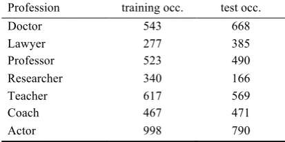
Figure 1. Variation between training and test We have noticed a great variation in the be-havior of the two systems. In order to search for an explanation for this difference we have looked at the distribution in the two corpora of the Named Entities, of the words denoting profes-sions and of the meta-contextual information - e-mails, urls, phones, and addresses. It turns out that these types of contextual information are distributed between training and test approxi-mately evenly. (see Table 1a,b).
Profession training occ. test occ.
Doctor 543 668
Lawyer 277 385
Professor 523 490
Researcher 340 166
Teacher 617 569
Coach 467 471
[image:3.595.311.518.458.561.2]Actor 998 790
Table 1a. Profession words in training and test
Address training occ. test occ.
Phone 1,109 1,169
Fax 606 426
e-mail 3,134 2,186
Table 1b. Meta-Context in training and test
[image:3.595.308.521.586.639.2]name is, on average, higher in test than in train-ing. The results plotted in Figure 1 show that it is not a question of which algorithm is better, but rather that there are different cases where one approach is preferred over the other. The prob-lem we face is deciding when it is appropriate to use one or the other.
To induce from the corpus itself when a piece of context is or is not a relevant context requires deep ontological inferences and a very powerful tool of semantic analysis of the context. Consider for example two words denoting profession, “doctor” and “researcher”, and their possible modifiers “internist”, “neurosurgeon”, and “pro-fessor” and “PhD”. In the first case it is certain that the coreference is not possible, while in the second the coreference is very probable. To find out such relationships is computationally very hard. However, the analysis carried out further shows that we can avoid making such computa-tions in most of the cases.
The number of different persons is a parame-ter that cannot be known beforehand. However, not all the names behave alike with respect to coreference. There are noticeable differences between names; for example less than 5 000 first names cover approximately 96% of the total of first names, while for the same percentage of coverage more than 70 000 of last names must be considered (Popescu et al. 2007). Let us call per-plexity of a name the number of different persons that carry it. The search space depends directly on the name perplexity. The bigger the perplex-ity, the larger the amount of information required for the correct coreference must be. It seems natural that the amount of contextual evidence required by a PCDC depends on the name per-plexity.
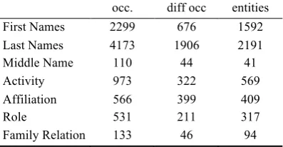
In order to evaluate the relationships between the context and the name perplexity, we need an annotated corpus. We have used the I-CAB cor-pus (Magnini et al. 2006), which is a four-day news corpus fully annotated, coreference rela-tionships included. The documents in this corpus are entire pieces of news. For each PNM we have counted how many contexts containing specific information about the person carrying the respec-tive name is present in that particular document. There are many types of contexts that refer to a person, but some of these types are very infre-quent. We considered only those types of infor-mation that are present at least 5% of the times in the context surrounding a PNM. Table 2 presents the results of this investigation.
occ. diff occ entities
First Names 2299 676 1592
Last Names 4173 1906 2191
Middle Name 110 44 41
Activity 973 322 569
Affiliation 566 399 409
Role 531 211 317
[image:4.595.317.516.72.175.2]Family Relation 133 46 94
Table 2. Name perplexity and context
On the second column the total number of oc-currences is listed, on the third column how many of these occurrences have different values (no case sensitive string match), and on the fourth column the number of different persons (Entities) having that information. The entries “activity”, “affiliation”, and “role” represent pieces of context where the respective informa-tion is directly expressed (no inferences). We call this type of context professional context and for approximately 30% of the PNMs, one of the above three types of professional contexts is pre-sent.
The perplexity of the first names, computed as the ratio between the fourth column and the third column is two times bigger than the perplexity of the last names. The lowest name perplexity is obtained by the names having a middle name - a name with at least three tokens – and it is very close to 1 (1.07). Comparatively, the highest per-plexity of two tokens name is 3. The relationship between the number of tokens of a name and its perplexity is straightforward: for names with more than four tokens the perplexity is 1 in 99,6% of the cases (the name by itself is a rele-vant context for coreference).
In approximately 74% of the cases there is just one entity corresponding to a two-token name. Considering any two PNMs of the same name the similarity of two of the professional contexts guarantees the correct coreference. However, two professional contexts are present in only 4% of the cases. There are just four cases when con-sidering just one professional attribute was mis-leading, and all these cases are high perplexity names. Moreover, in the case of many low per-plexity names, the contexts could be minimally similar in order to correctly corefer any two PNMs of that respective name.
fo-cusing on the exact figure for name perplexity, we will try to partition the names according to their perplexity and to link each partition to a specific behavior with respect to coreference. The partitioning technique should ensure that the variance of the name perplexity within the same partition is low and that a specific amount of context should lead to the correct coreference decision for the great majority of names within that partition.
Our working hypothesis is that we can esti-mate the name perplexity within each partition and use this information to control the amount of contextual evidence required. Let us recall the “John Smith” and “Barack Obama” example from the previous section. Both “John” and “Smith” are American common first and last names. The chance that many different persons carry this name is high. On the other hand, as both “Barack” and “Obama” are rare American first and last names respectively, almost surely many mentions of this name refer only to one person. The argument above does not depend on the context, but just on the prior estimation of the usage of those names. Having an estimation of a name’s perplexity, we may decrease/increase the amount of contextual evidence needed.
4
(p,
γ)Statistical Model
Let D be the set of all PNMs from a given corpus
C and let DN be the set of corresponding names. We want to find a partition P of DN such that within each partition the name perplexity varies only within predicted margins. Let X be a ran-dom variable with uniform distribution over DN
and let Y be the random variable defined by X’s name perplexity. Let us suppose that we want P
= {p1, p2, …, pm} to be a partition of DN, where
the percentage of each partition class is pi:the
first partition class contains p1 percentage of the
name population, the second partition class con-tains p2 percentage of the name population and
the last partition class contains pm = 1 -
Σ
piper-centage of the name population.
If we knew the distribution function of Y, let’s call it F, we would simply determine ξi from
equation 1, where Pi =
Σ
pk , k ≤ i :ξi = F-1(Pi)⇔ F(Y<ξi) = Pi (1)
and we would know that in each partition pi the
name perplexity is between ξi-1 andξi, with ξ0 = 0.
However we do not know F. Fortunately, we can estimate ξi.
There is no restriction that may impose a par-ticular form for F; for example, the normal dis-tribution hypothesis of name perplexity is ruled out by a χ2 test with 96.5% confidence for the 14
names chosen from WePS-1 (see Section 3, first paragraph).
We are going to present a distributional free method for constructing the partition P. The ad-vantage of this method is that it does not depend on any assumption about the PNMs distribution.
Let us consider X1, X2,…, Xn a sample of
in-dependent and identical distributed names from
DN. By rearranging the indexes, without losing the
generality, let us suppose that Y1, Y2, …, Yn is
ordered, that is Y1≤ Y2≤ … ≤ Yn. Even if we do
not know what form F has, we can still use equa-tion (1) in order to estimate ξi. The expected
value of F(Yi) is (Hogg, Mckean, Craig 2006):
E[F(Yi)] = i/(n+1) (2)
which is an estimation of how much mass prob-ability is on the left of Yi. In our terms, we
esti-mate that E[F(Yi)] percentage of the name
popu-lation has a name perplexity lower than Yi.
For a given number ξ, the percentage of the
name population having the name perplexity at most ξ is determined by finding the smallest Yi
greater thanξ and use the equation (2) to
esti-mate E[F(Yi)].
In order to build the partition P we are inter-ested in the percentage of the name population that has the perplexity between two given values. Let (Yi, Yj) be the smallest interval that includes
these two values. We can estimate the percentage of the name population that has a perplexity be-tween Yi and Yj. This estimate is simply F(Yj) –
F(Yi). We can use directly equation (2) to
esti-mate this difference. However, it is more impor-tant to have a confidence interval for this esti-mate, that is we want to know what the probabil-ity is that the interval (F(Yi), F(Yj)) contains at least a given percentage of the population, p. The optimal partition P is the one that maximizes the confidence in the fact that within each of the par-tition classes as many names as possible have the name perplexity in a given interval.
Let p be a given real number between (0,1) representing the mass probability that goes into the interval (F(Yi), F(Yj)). Let γ = P(F(Yj) –
F(Yi) ≥ p). Fortunately γ has a distribution that
does not depend on F. More precisely, γ has a
γ = P(F(Yj) – F(Yi) ≥ p) =
∫
p1 Γ(n+1)/( Γ(j-i)) Γ(n-j+i+1)xj-i-1(1-x)n-j+idx (3)The Γ, called the gamma function, is the
ex-tension of the factorial, Γ(x) =
∫
0∞tx-1e-tdt. Thegamma function has the property that Γ(x) = Γ
(x-1) Γ(x-2)…. Γ(1); for x an integer, as the
argu-ments in the formula (3) are, Γ(x) = (x-1)!
The formula (3) gives us a method of building the partition P. Let us start with a set of perplex-ity intervals: (ξ0, ξ1], (ξ1,ξ2], …(ξm-1, ξm]. We
partition the names in DN such that we maximize the confidence γ that at least pi percentage of the
name population has a name perplexity in (ξi-1, ξi]. We chose an independent and identical
dis-tributed sample X of names to which the ordered sample Y of name perplexity values corresponds. We start with the lowest perplexity interval and determine p1,γ1 and Y0, Yi1, such that Y0≤ξ0 ≤ξ1 ≤Yi1 and γ1 = P(F(Yi1) – F(Y0) ≥ p1). The ith
in-dex varies according to the desired γ1, whenp1 is
given,and vice-versa. We can choose i1 with m-1 liberty grades. Once we are satisfied with the values (p1,γ1), we search for the i2th index such
that Yi1 ≤ ξ1 ≤ ξ2 ≤Yi2 and (pi2,γi2) have the
de-sired value. The process continues till the penul-timate (pm-1,γm-1). We have no liberty in choosing
the (pm,γm).
We can compute the size of the sample needed for guaranteeing a minimum γ and p.
Let us give an example. Suppose that (ξ0, ξ1] =
(0,2]. Thus we are interested in finding p, the percentage of the name population such that we can be γ sure that at least p names have a
per-plexity between 1 and 2 inclusive. We take a random sample of n = 30 and suppose the small-est index i1 such that Yi≥ 3 for all i > i1 is 17 .
We want to compute the confidence γ that at
least p = 60% of the name population has the name perplexity within (0,2]:
γ = 1 -
∫
0 0.6 30!/(16!15!)x15(1-x14)dx == 1 – k(
∫
0 0.6 x15dx +∫
0 0.6 x29dx) == 1 – k[(1/16)(6/10)16 + (1/30)(6/10)30]
≥ .965
In practice we want to have optimal values for p and γ; a large p implies a small γ and vice-versa. The optimality is determined by the accu-racy of the CDC system: we want to have the
largest possible percentage of names into each partition such that our confidence that the names inside each partition have the same perplexity.
It is useful to work the equation (1) back-wards. Suppose that we established the first par-tition class of P - we have found the i1th index, p1, and γ1. Now we refer only to the names in the
partition class. We can compute the probability that a certain percentage of the names within that particular partition class have a given name per-plexity. That is, we consider a random sample inside the partition class, X, and its correspon-dent random variable Y, as above. The confi-dence that p1inside percentage of names have the
name perplexity ξp within the interval (Y0, Yith)
is:
P(Y0 < ξp <Yi1) =
Σ
k (kn) pk(1-p)n-k (4)(kn) represents the k-combinations of size n.
By taking advantage of the bootstrapping method (Efron and Tibshirani 1993) we do not have to resample inside the partition class. We use the Y0, .., Yi1 values with replacement. Using
(4) we obtain p1inside which shows us which
per-centage inside the partition class has the name perplexity within (Y0, Yi1]. And consequently we
can compute γ1inside. Finally we are able to
formu-late the following statement about each partition class:
In the ith partition class enter pi
percent-age of the name population with a confi-dence γi.Insidethis partition class we are γiinside confident that piinside percentage of
the names have a name perplexity within (Yi1-1, Yi1].
The p and
γ
indicate the theoretical values
that define the partition. In practice the exact
distribution of the names into the subset is
unknown, therefore each heuristics that
computes the perplexity creates its own
dis-tribution. The values
γ
iinsideand p
iinsidecontrol
how much a certain heuristics departs from
the theoretical values. The optimal heuristics
have very big figures for
γ
iinsideand p
iinside.
In the next section we present an
experi-ment carried on a news corpus. We show
how the above model leads to a stable
parti-tion of names and that inside each partiparti-tion
5
Name Perplexity Partition
For the experiment described in this section, we have used a two-year part of the seven-years Ital-ian local newspaper corpus called Adige500k Corpus (Magnini 2006).
We describe below how we compute the per-plexity class for the one-token names and two-tokens names respectively. As mentioned in sec-tion 3, the name perplexity decreases rapidly for tree-token or more names. If desired, the same technique could also be applied for those names. In Adige500k there are 106, 187 different one-token names; 429, 243 two-one-token names; 36, 773 three-token names; 5, 152 four-token names, 940 four token names and less than 300 different four-token or more names.
An estimate of the name perplexity of the one-token names is the size of the different one-one-token names with which it forms a complete PNM in the corpus. For example for the first name “John” the estimation of its perplexity is the size of the one-token last names it combines with in forming PNMs, like “Smith, Travolta, Kennedy” etc. The bigger the size of its complementary names, the higher is its name perplexity. In Table 3 we present the figures of these estimates.
occurrences (interval) average perplexity
1-5 4.13
6-20 8.34
21-100 17.44
101-1,000 68.54
1,000-5,000 683.95
5,000-31,091 478.23
Table 3. Average perplexity one-token names
We start with a five name perplexity classes: “very low” (VL) , “low” (L) , “medium”, (M) “high” (H) and “very high” (VH). The name per-plexity of a two-token name is interpolated from the name perplexity of its components. We used the following heuristics: the name perplexity class is the average name perplexity classes of its one-token name. If the name perplexity classes are the same then the name perplexity class of the whole name is one class less (if possible).
In order to compute the borderline
be-tween two consecutive classes we apply the
(p,
γ
) method. We selected 25 two-tokens
names and we manually investigate their
oc-currence in order to know their real name
perplexity. The perplexity classes obtained
after applying the (p,
γ
) technique are listed
in Tables 4a and 4b respectively.
perplexity class percentage
very high (VH) 5.3%
high (H) 8.7%
medium (M) 20.9%
low (L) 27.6%
very low (VL) 37.5%
Table 4a. First Name perplexity classes
perplexity class percentage
very high (VH) 1.8%
high (H) 3.36%
medium (M) 17.51%
low (L) 20.31%
very low (VL) 57.02%
Table 4b. Last Name perplexity classes
Tables 4a and 4b fully describe the partition for one-token names. Ordering the one token names according to their perplexity we chose the first ones according to the percentage listed above. The same process applies to the one-token last names. The values computed for two-token names are listed.
P γ pinside γinside
VH 0.04% 70% 70% 80%
H 2.53% 76% 70% 80%
M 10.08% 87% 80% 82%
L 27.97% 90% 99% 90%
VL 59.38% 96.5% 99% 96.5%
Table 5. (p, γ, pinside,γinside) values
6
CDC with Name Perplexity Estimates
The working hypothesis is that using the name partition obtained with the (p,γ
) procedure we
can effectively improve the accuracy of a
CDC system by reducing/increasing the
amount of contextual evidence required for
coreferencing according to the perplexity
class to each the name belong.
combin-ing the names in 6a and 6b are found in the
corpus, we consider 11 other two-tokens
names having the same distribution. On the
first column the names are listed, on the
sec-ond column the computed perplexity (P), on
the third column the number of occurrences
as one-token name (O), on the fourth the
number of occurrences in a two-token name
(T) and on the last column the computed
perplexity class (PC).
Name P O T PC
Dellai 7 31091 10722 VL
Parolari 171 1,619 2207 H
Prodi 52 9184 3382 M
Ruini 15 554 203 L
[image:8.595.70.287.219.424.2]Rossi 753 7506 8356 VH
Table 6a. Test Last Names
Name P O T PC
Camillo 276 664 1731 L
Lorenzo 2088 2167 2198 H
Paolo 5255 4001 51244 VH
Romano 14 886 6414 M
[image:8.595.315.512.257.386.2]Varena 5 10 85 VH
Table 6b. Test First Names
We compare the results obtained by our
CDC system using the name perplexity
parti-tion (S) against two baselines: one that
con-siders only the context at the sentence level
and (BLS) one that considers the whole news
(BLN). We obtain the following figures
us-ing the B-CUBED measure: S scores .72,
BLS .59 and BLN .61. The gain in accuracy
of more than 10% is due to the use of name
perplexity classes.
The great advantage of using the (p,
γ
)
es-timates can be seen in those case where the
ratio between the number of mentions and
the rank of the name is close to extremes:
either big number of mentions and low name
perplexity, or low number of mentions and
high name perplexity. In the first case the
contextual evidence for coreference may be
very scarce and in the second case, the
re-quirement for strong contextual evidence is
the best decision. Our results suggest that
loosening the contextual requirements in the
first case leads to an important gain in recall,
up to 40%, while the lose in precision is less
than 1.5%. The situation is best described by
four panels of the five-number-summary
plots of the test corpus. Panel A shows the
distribution of the main five quantilies
con-sidering all the names together. Panel B
shows the distribution for very low
perplex-ity class, Panel C for medium perplexperplex-ity
class and Panel D for the very high
perplex-ity class. The number of outliers in Panel A
is high, which makes it difficult for any CDC
system, but inside each perplexity class the
variation is reduced.
7
Constructing an Evaluation Corpus
The (p, γ) technique could be used for
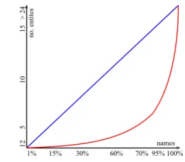
construct-ing a test corpus for the CDC task. The main problem faced in the construction of the test cor-pus is data variation. The number of different entities mentioned with the same name is a ran-dom variable with a big variance. The distribu-tion of the number of entities is very skew. The average perplexity is 2.01%, but less than 18% of the total number of names have a perplexity greater than 3. In Figure 2 we plot a modified Lorenz curve (the vertical axis is not divided in percentage, as the values are discrete).
[image:8.595.346.481.573.691.2]the expectation is that in such corpus, the aver-age perplexity is very low, and consequently, the great majority of cases can be coreferenced by a simple algorithm. Therefore, this test corpus may be largely ineffective in ranking the algorithms. In fact, we want to construct an evaluation cor-pus that is able to promote the most effective algorithms. The discriminative power of a test corpus is directly related to the variance of the data. Moreover, if only certain names are consid-ered for a test corpus, the variance can be very low; in particular, when the test corpus contains just one name the variance is zero. It is difficult to see the merits of different algorithms when tested on such corpora.
In order to make more informative statements we need to construct an evaluation corpus that is less dependent on the data variance. A possible solution is to form a partition of the set of the PNMs, that is, to split the whole set of PNMs in mutual disjunctive groups. This type of method-ology is called stratified sampling, mainly be-cause each group is a stratum. The sampling strategy, the number of sampling elements, the variance and the sampling error can be calculated independently for each strata.
The main advantages of stratified sampling are that we can concentrate on the special groups, that in general this strategy improves the accuracy of the estimation, and that the number of elements in each stratum can be conveniently chosen. The main disadvantages are related to the difficulty in finding a suitable partition of the population. The strata should be chosen prior to the sampling time, but the homogeneity inside the stratum should be guaranteed.
Our proposal is to use the name perplexity in-tervals. We argue that this proposal is four-fold sustainable. Firstly, the name perplexity is di-rectly connected to the random variable whose distribution we estimate, namely the number of entities. Secondly, for free names it can be com-puted off - line. Thirdly, it gives us an independ-ent and formally correct way to make a partition. Fourthly, it easily allows a separation between the important and unimportant cases.
To begin with, let us suppose we have a name that has n occurrences in the Adige 500K. If n is relatively large, than we can be sure that there are some dominant entities that may be repre-sented by the majority of PNMs that have this name as value. However, it is unknown whether the n comes from the fact that there are indeed some dominant entities or whether the name by itself is a frequently used name.
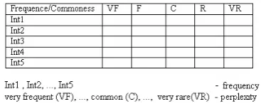
In order to deal with the differences between frequency vs. perplexity, we propose to build a matrix defined by the frequency classes as rows and perplexity classes as columns. In Figure 3 we present this matrix.
Figure 3. Frequency/Commonness strata ma-trix.
The number of different names in each of the cells of the matrix may differ according to the departure of the normal distribution of each stra-tum. In general, if the real distribution is normal, then as much as ten examples are sufficient. Oth-erwise, for not very skew distributions, which we expect most of the strata to have, an average of 30 examples should suffice. In same cases, as the normal distribution can be appropriately sampled when both Np and N(1-p) are grater than five – where p is the ratio perplexity/frequency and N the sample dimension – the number of elements in the cell may be around 200, by a maximal rough estimation.
8
Conclusion and Further Research
We have presented a distributional free statistical method to design a name perplexity system, such that each perplexity class maximizes the number of names for which the prior coreference prob-ability belongs to the same interval. This infor-mation helps the PCDC systems lower/increase adequately the amount of contextual evidence required for coreference.
The approach presented here is effective in dealing with the problems raised by using a simi-larity metrics on contextual vectors improving the overall accuracy with more than 10%.
We would like to increase the number of cases considered in the sample required to delimit the perplexity classes. Equation (3) may be devel-oped further in order to obtain exactly the num-ber of required cases.
The (p, γ) procedure is effective is dealing
[image:9.595.329.513.145.218.2]Acknowledgments
The corpus used in this paper is Adige500k, a seven-year news corpus from an Italian local newspaper. The author thanks to all the people involved in the construction of Adige500k.
References
J. Artiles, Gonzalo, J., S. Sekine. 2007. Establishing a benchmark for WePS. In Proceedings of Se-mEval.
A. Bagga, B. Baldwin. 1998. Entity-based Cross-Document Co-referencing using the Vector Space Model. In Proceedings of ACL.
J. Chen, D. Ji, C. Tan, Z. Niu. 2006. Unsupervised Relation Disambiguation Using Spectral Cluster-ing.In Proceedings of COLING
C. Gooi, J. Allan. 2004. Cross-Document Corefer-ence on a Large Scale Corpus. In Proceedings of ACL.
R. Grishman. 1994. Whither Written Language Evaluation? In Proceedings of Human Language Technology Workshop, pp. 120-125. San Mateor. E. Elmacioglu, Y. M. F. M.Y.Khan, D. Lee. 2007. PSNUS: Web People Name Disambiguation by Simple Clustering with Rich Features, in Proceed-ings of SemEval
H. Han, W. Xu. 2005. A Hierarchical Bayes Mix-ture Model for Name Disambiguation in Author Citations, in Proceedings of SAC’05
R. Hog, J. McKean, A. Craig, 2006. Introduction of Mathematical Statistics, ed. Prentice Hall
E. Lefever, V. Hoste, F. Timur. 2007. AUG:A Com-bined Classification and Clustering Approach for Web People Disambiguation, In Proceedings of SemEval
B. Magnini, M. Speranza, M. Negri, L. Romano, R. Sprugnoli. 2006. I-CAB – the Italian Content An-notation Bank. LREC 2006
V., Ng. 2007. Shallow Semantics for Coreference Resolution, In Proceedings of IJCAI
T. Pedersen, A. Purandare, A. Kulkarni. 2005. Name Discrimination by Clustering Similar Contexts, in Proceeding of CICLING
O. Popescu, C. Girardi. 2008. Improving Cross Document Coreference, in Proceedings of JADT
O. Popescu, B. Magnini. 2007. Inferring Corefer-ence among Person Names in a Large Corpus of News Collection, in Proceedings of AIIA
Y. Wei, M. Lin, H. Chen. 2006. Name Disambigua-tion in Person InformaDisambigua-tion Mining, in Proceedings of IEEE