Probabilistic sensitivity analysis for multivariate model outputs with applications to Li ion batteries

PAPER • OPEN ACCESS

Probabilistic sensitivity analysis for multivariate

model outputs with applications to Li-ion batteries

To cite this article: V. Triantafyllidiis et al 2018 J. Phys.: Conf. Ser. 1039 012020

View the article online for updates and enhancements.

Related content

Uncertainty Quantification in Solidification Modelling

K Fezi and M J M Krane

-Parameter Identification of Equivalent Circuit Models for Li-ion Batteries Based on Tree Seeds Algorithm

W J Chen, X J Tan and M Cai

-A review on prognostics approaches for remaining useful life of lithium-ion battery

-Content from this work may be used under the terms of theCreative Commons Attribution 3.0 licence. Any further distribution

Probabilistic sensitivity analysis for multivariate

model outputs with applications to Li-ion batteries

V. Triantafyllidiis1, W.W. Xing1, P.K. Leung2, A. Rodchanarowan3, and A.A. Shah1

1_{School of Engineering, University of Warwick, Coventry CV4 7AL, UK} 2_{Department of Materials, University of Oxford, Oxford, OX1 3PH, UK}

3_{Department of Materials Engineering, Faculty of Engineering, Kasetsart University, 50} Ngamwongwan Rd., Ladyao, Chatuchak, Bangkok, 10900, Thailand

Abstract. Full battery models are highly complex, which limits their application to tasks such as optimization and uncertainty quantification. To lower the computational burden, sensitivity analysis (SA) can be used as a precursor to identify the most important parameters in the model, but SA itself relies on a high number of full model evaluations, which has motivated the use of emulators. For high-dimensional output problems, emulators are challenging to construct. In this paper we develop a probabilistic framework for SA of high-dimensional output models using a Gaussian process emulator based on dimensionality reduction. This allows us to perform SA under uncertainty for multi-ouput problems, providing error bounds for the emulator predictions of sensitivity measures. We show how this can be achieved using Monte Carlo sampling or possibly by using semi-analytical expressions with highly efficient sampling. Moreover, we can perform SA for multivariate outputs by ranking the sensitivity measures related to (uncorrelated) coefficients in a basis for the output space.

1. Introduction

The large number of parameters appearing in mathematical models and numerical codes for batteries complicates modelling efforts. Lowering the time cost of simulations by identifying the most influential parameters and studying their effects is an effective precursor to tasks such as design optimization and uncertainty quantification (UQ). This process is referred to assensitivity analysis (SA) [1]. SA methods can be categorized in different ways. In quantitative SA the influence of a parameter (usually referred to as “factor” of aninput) is assigned (reproducibly) a number called a sensitivity index orimportance measure. Inlocal SA, the output variability is studied by perturbing an input around a nominal (base) value, while methods that attempt to measure the output variability across the entire input space are termed global. For small variations in the inputs local methods may be more computationally efficient. In many cases involving complex nonlinear models, however, local SA methods are inadequate.

In the context of battery models, very little attention has been paid to SA. In the majority of cases, formal SA methods are not used; the model is simply run multiple times by varying factors individually and inspecting the outputs, using ad-hoc measures or by employing visualization tools [2]. In a small number of studies more rigorous approaches have been used, but almost invariably with highly simplified models. Applying formal SA methods to complex battery and fuel cells models is computationally burdensome and often not feasible, particularly with brute force Monte Carlo (MC) approaches. In order to overcome this issue an emulator or meta-model can be used. The emulator itself can be difficult to construct when the input and/or output space is high-dimensional (e.g., input and/or output fields). If the quantity of interest (QoI), which is derived from the output, is a scalar, an alternative is to use an emulator directly between the inputs and QoI. It may be the case, however, that there are multiple QoIs, in which case it would be ideal to emulate the output, especially when other tasks (e.g. UQ) involving different quantities, including perhaps the original output, are to be performed subsequently.

To address these issues, we develop an approach for SA of a nonlinear Li-ion battery model by employing a Gaussian process emulator based on dimensionality reduction to approximate entire charge-discharge curves. QoIs are extracted from the curves in order to perform a SA. We show how it is possible to perform an efficient probabilistic SA in the context of a variance-based approach [4], extending previous results for the scalar case considered by Oakley and O’Hagan [5] to linear functional QoIs derived from the multi-dimensional output. Lastly, using the emulation method we are able to perform a SA of multiple outputs (including in high dimensional spaces) by ranking coefficients in a low-dimensional subspace approximation of the output space.

2. Problem setup and sensitivity analysis

Suppose that the model output isy=η(x;ξξξ)∈ F for some function spaceF, wherexrepresents, e.g., space, time or space-time and ξξξT = (ξ₁, ξ₂, ..., ξ_k) ∈ X ⊂ Rk is a vector of input factors; that is, a spatial, temporal or spatio-temporal field, parameterized by inputsξξξ. The computer model (simulator), on the other hand, provides a finite-dimensional approximation of η(x;ξξξ), e.g., at a finite number of points in a spatial and/or temporal grid or in terms of a finite basis. We may write the simulator output as a vector y∈Rd, in which dis the number of degrees of freedom, e.g., thedcomponents ofyrepresent values of η(x;ξξξ) atdpointsx. We can therefore consider the simulator as a mapping ηηη :X → Y ⊂ Rd _{between a feasible input space X ⊂ R}k

and an output space Y, i.e., y=ηηη(ξξξ).

Let Q be a scalar QoI that is derived from y via a linear functional G :F → Q ⊂ R. We can instead consider Q as a mapping F = (G◦η)(ξξξ) :ξξξ → Q directly between X and Q, i.e.,

Q=F(ξξξ) =G(η(x;ξξξ)). In reality, we have an approximationq=f(ξξξ) of Q, where the mapping

f :X → Qis derived from a linear functionalg:Rd_{→ Q ⊂Rthat acts on the simulator outputs} y, that is f(ξξξ) = (g◦ηηη)(ξξξ) =g(ηηη(ξξξ)). We develop a SA framework in which the outputs yare estimated by an emulator. We first describe the SA methods employed and the construction of the emulator. We then show how it is possible to perform SA on QoIs derived from the emulator output, before presenting a probabilistic SA analysis and a method for multi-output SA.

One approach to SA measures the sensitivity of the QoI by estimating the derivative ∂_ξif

around a nominal (base) point ξξξ using finite differences [6]. The main weakness of such local methods is that they provide no information on how the sensitivity to a given ξ_i depends on the values of the other factors. In order to extend this method to a global analysis we may use multiple base points {ξξξ_j}r

j=1, which leads to the class of elementary effect tests (EETs).

Suppose thatX is the unit hypercube, and each direction ξ_i is discretized intoplevels (points). The elementary effect of ξ_i atξξξ_j = (ξ_j,1, . . . , ξ_j,k)T _{is: ‘}

where Δ_i ∈ {1/(p−1), . . . ,1−1/(p−1)}. Typically, Δ_i = Δ, ∀i. Morris [3] proposed two sensitivities measures for each ξ_i, namely the mean and the standard deviation of the finite distributionF_i over{EE_i(j)}r_j=1 (or|EE_i(j)|). The meanμ_i of EE_i measures the influence of ξ_i, while the standard deviation σ_i measures the degree of interaction with the other factors.

To calculate the statistics for each elementary effect, i.e.,μ_i andσ_i, we can randomly choose

M base points{ξξξ_j}M

j=1, then construct so-calledtrajectories inX ofk+1 pointsξξξj∪{ξξξj,n}kn=1 for

each j. Settingξξξ_j,0 =ξξξ_j, the trajectory point ξξξ_j,n is obtained by perturbing a randomly chosen factor of ξξξ_j,n−1 by ±Δ until all factors have been perturbed, but with the property that ξξξ_j,n

andξξξ_j,n−1 differ in only one factor. The model is run at every point in each of the trajectories (a total of M(k+ 1)) to obtainEE_i,j,i= 1, . . . k,j = 1, . . . M, yielding estimates of μ_i and σ_i. A more sophisticated approach to SA, embedded in probability, involves treating the inputs as stochastic variables, which leads to a distribution over the QoI [4, 6]. A variance based first-order effect of each input factor is given by Var_ξi(E_ξξξ∼i[q|ξ_i]), where E[·] and Var(·) denote expectation and variance operators with respect to the distribution over a subscripted random variable; or with respect to the distributionp(ξξξ) overξξξif no subscript is present, i.e. E[·]≡E_ξξξ[·]. The quantity ξξξ_∼i is the vector of all inputs factors excluding ξ_i (and similarly for multiple indices). The first order sensitivity index (or main effect index) for the input ξ_i is defined as

S_i ≡ Var_ξi(E_ξξξ∼i[q|ξ_i])/Var(q), which measures the contribution of the main effect of ξ_i to the total QoI variance. Another measure of sensitivity, defined below, is thetotal effect index, which incorporates interactions between the factors ξ_i:

S_Ti ≡E_ξξξ∼i[Var_ξi(q|ξξξ_∼i)]/Var(q) = 1−Var_ξξξ∼i(Eξ_i[q|ξξξ_∼i])/Var(q). (2)

The variance-based SA framework can be couched in terms of the decomposition of the variance of q. Suppose q =f(ξξξ)∈L2(X) (square integrable functions defined onX) and X is (without loss of generality) a unit hypercube X ={ξξξ|0≤ξ_i ≤1;i= 1, . . . , k}. We also assume that the factors are independently and uniformly distributed within X, so that the probability density functions satisfy p(ξ_i1, . . . , ξ_il) = 1_[0,1]l for {i₁, . . . , i_l} ⊂ {1, . . . , k}, where 1_A is the indicator function on a set A. The expectation operators E_ξξξ∼i

1...il[·] are then unweighted integrals over

ξ_i1, . . . , ξ_il. The functionf(ξξξ) can be decomposed in the following way (Hoeffding [7]):

f(ξξξ) =f₀+

k

i=1

f_i(ξ_i) +

k

i=1 k

j=i+1

f_ij(ξ_i, ξ_j) +. . .+f_1...k(ξ₁, . . . , ξ_k), (3)

where f₀ is a constant, f_i(ξ_i) (the main effect of ξ_i) is a function only of ξ_i,

f_ij(ξ_i, ξ_j) (the interaction) is a function only of ξ_i and ξ_j, and so on. The condition ₁

0 fi1i2...is(ξi1, ξi2, . . . , ξis)dξiw = 0 is imposed for 1 ≤ i1 < i2 < . . . < is ≤ k and

i_w ∈ {i₁, i₂, . . . , i_s}[7]. Thus, the summands are orthogonal, in the sense that:

X

f_i1i2...im(ξ_i1, ξ_i2, . . . , ξ_im)f_i

1i2...in(ξi1, ξi2, . . . , ξin)dξξξ= 0, (4)

for{i₁, i₂, . . . , i_m} ={i₁, i₂, . . . , i_n}. Moreover,f₀=E[q] =_Xf(ξξξ)dξξξ,f_i=E_ξξξ∼i[q|ξ_i]−f₀,f_ij =

Eξξξ∼ij[q|ξi, ξj]−fi−fj−f0, etc.. By squaring and integrating Eq. (3) and using the orthogonality

property, we obtain a decomposition of the total variance V = Var(q) =_Xf2(ξξξ)dξξξ−f₀2, that is,V =k_i=1V_i+k_i=1k_j=i+1V_ij+. . .+V_1...k, in whichV_i=Var_ξi(f_i(ξ_i)) =Var_ξi(E_ξξξ∼i[q|ξ_i]),

define higher order sensitivity indices by normalizing the V_i1...il, e.g. the second-order index

S_ij =V_ij/V, which measures the effect of interactions between ξ_i and ξ_j on q.

The main and total indices can be computed using a quasi MC method [1] by first generating a matrix X = [ξ_i,j], i = 1, . . . ,2k, j = 1, . . . , N, of N points in the 2k hypercube, using a low-discrepancy sequence such as a Latin hypercube. This is done according to the distribution

p(ξξξ) over the factors, e.g.,p(ξξξ) =1_[0,1]k for independentξ_i ∼ U[0,1]. Xis then partitioned into a matrixA∈RN×k consisting of the first k columns and a matrix B∈RN×k consisting of the remaining kcolumns. This provides two independent sets of N samples in the khypercube. A third matrix C_i consists of the columns of matrixBexcept thei-th column, which is set to the

i-th column ofA. The next step is to compute the QoI q by running the model at the selected inputs contained in the sample matricesA,B, andC_i to yields vectors q_A=f(A),q_B =f(B) and q_Ci =f(C_i) (f(A) is used to denote vectorizedq values from the set consisting of the rows of A). The indices S_i and S_Ti are then estimated as follows:

S_i = (1/N)

_N

j=1qA,jqCi,j−f02

(1/N)N_j=1q2_A,j−f₀2 , STi =

(1/N)N_j=1q_B,jq_Ci,j−f₀2

(1/N)N_j=1q_A2_,j−f₀2 , (5)

where q_A,j is the j-th coordinate of q_A (etc.) and f₀ = (1/N)N_j=1q_A,j is the sample mean. This procedure is repeated for each i = 1, . . . , k. The first of Eqs. (5) follows from the basic definition Var_ξi(E_ξξξ∼i[q|ξ_i]) = _[0,1]E2_ξξξ

∼i[q|ξi]dξi−(

[0,1]Eξξξ∼i[q|ξi]dξi)2. The last term is E2[q] =

f₀2, while the first term can be written as: _[0,1]E2_ξξξ

∼i[q|ξi]dξi =

[0,1]k

[0,1]k−1f(ξ1, . . . , ξk) ×

f(x₁, . . . , x_k)dξξξdξξξ_∼i, i.e., the expectation over ξξξ and ξξξ_∼i of f(ξ₁, . . . , ξ_k)×f(x₁, . . . , x_k), which explains the MC estimate in Eq. (5). A similar explanation can be given for the S_Ti estimate.

The cost of this procedure is 2N runs of the model to generate the matricesAandB, and an additionalN kruns to obtain the QoIs corresponding toC_i. This give a total ofN(k+2), which is much lower than the cost of brute-force MC estimates ofVar_ξi(E_ξξξ∼i[q|ξ_i]) andVar_ξξξ∼i(E_ξi[q|ξξξ_∼i]). The former, e.g., would requireO(N) runs (N k) to estimate the inner expectation for a fixed

ξ_i, which we would be repeated O(N) times to estimate the outer variance, leading to O(N2) runs for each i.

3. Gaussian process emulation of the model outputs

Suppose we are given training points {y_j}m_j=1 ⊂ Y, which are values of y=ηηη(ξξξ) at the design points {ξξξ_j}m

j=1. Without loss of generality we mean centre the training points: yj → yj −y,

where y = m_k=1y_k. Assume that Y is a low-dimensional linear subspace of Rd. We derive an approximate basis for Y using principal component analysis (PCA) [8], i.e., we find a linear transformation w(ξξξ) = VTy, in which V ∈ Rd×d has orthogonal columns v_i (a basis for Rd) and the uncorrelated components w_i(ξξξ) ofw(ξξξ) have decreasing variance with i.

Let Σ = E[yyT] be the symmetric and positive definite variance-covariance matrix. The eigenvalue problemΣv=λvyields thev_iand corresponding positive eigenvaluesλ₁ >· · ·> λ_d. The components of a point in this basis satisfyVar[w_i(ξξξ)] =λ_i andE[w_i(ξξξ)w_j(ξξξ)] = 0 fori=j. Any point y ∈ Y can be written in the form y =Vw(ξξξ) =d_i=1w_i(ξξξ)v_i =d_i=1(vT_i y)v_i and an r-dimensional approximation y_r ∈ Y_r = span(v₁, . . . ,v_r) of y is given by y_r = V_rw_r(ξξξ) = _r

i=1wi(ξξξ)vi, whereVr= [v1. . .vr] and wr(ξξξ) = (w1(ξξξ), . . . , wr(ξξξ))T. It can be demonstrated

Let us focus onw_i(ξξξ) for somei∈ {1, . . . , r}. We wish to approximate w_i(ξξξ) :X →Rgiven values of this function (from a PCA) at design points {ξξξ_j}m_j=1. In GPR, we place a GP prior distributionindexed byξξξ∈ X overw_i(ξξξ). The distributionp(w_i(ξξξ₁), . . . , w_i(ξξξ_m)) for an arbitrary finite collection of indices{ξξξ₁, . . . , ξξξ_m}is Gaussian. The GP prior isw_i(ξξξ)|θθθ_i ∼ GP(0, c(ξξξ, ξξξ;θθθ_i)), which has a zero mean function (we set w_i(ξξξ_j) → w_i(ξξξ_j)−w_i, where w_i = (1/m)_jw_i(ξξξ_j)) and a covariance functionc(ξξξ, ξξξ;θθθ_i), dependent uponhyperparameters θθθ_i. We employ a square-exponential function for all i: c(ξξξ, ξξξ;θθθ_i) = θ₀exp{−(ξξξ−ξξξ)Tdiag(θ_i,1, . . . , θ_i,k)(ξξξ−ξξξ)}, where

θθθ_i = (θ_i,0, . . . , θ_i,k)T, in which θ_i,1, . . . , θ_i,k are the inverse square correlation lengths.

The distribution of d_i ≡ (w_i(ξξξ₁), . . . , w_i(ξξξ_m))T given θθθ_i (i.e., the likelihood) is p(d_i|θθθ_i) = N(0,C_i), with covariance matrix C_i = [c(ξξξ_i, ξξξ_j;θθθ_i)]m_i,j=1. The predictive distribution at new inputsξξξ∈ X is obtained from the joint distribution p(w_i(ξξξ),d_i|θθθ_i) by conditioning on d_i [10]:

w_i(ξξξ)|d_i, θθθ_i ∼ GPm_i(ξξξ), c_i(ξξξ, ξξξ) ,

m_i(ξξξ) =c_i(ξξξ)TC_i−1d_i+w_i, c_i(ξξξ, ξξξ) =c(ξξξ, ξξξ;θθθ_i)−c_i(ξξξ)TC−_i 1c(ξξξ), (6)

in which c_i(ξξξ) = (c(ξξξ₁, ξξξ;θθθ_i), . . . , c(ξξξ_m, ξξξ;θθθ_i))T. The hyperparameters can be specified by point estimates [10] such as the maximum log likelihood estimate (MLE): θθθ_{i,M LE} = arg max_θθθi(−ln|C_i|/2 −dT_i C−_i 1d_i/2). This procedure is repeated for each i = 1, . . . , r to obtain w_r(ξξξ) = (w₁(ξξξ), . . . , w_r(ξξξ))T_{. Using MLE estimates, we obtain E[w}

r(ξξξ)] = m(ξξξ) ≡

(m₁(ξξξ), . . . , m_r(ξξξ))T. The predicted variance of each coefficient is Var(w_i(ξξξ)) = c_i(ξξξ, ξξξ). The model outputs are therefore distributed as follows (noting thatCov (w_i(ξξξ), w_j(ξξξ)) = 0 fori=j):

y_r−y=ηηη_r(ξξξ) =V_rw_r(ξξξ)∼ GPm_yr,c_yr(ξξξ, ξξξ)

m_yr(ξξξ) =E[ηηη_r(ξξξ)] =V_rm(ξξξ),

c_yr(ξξξ, ξξξ) =Covηηη_r(ξξξ), ηηη_r(ξξξ) =V_rdiag(c₁(ξξξ, ξξξ), . . . , c_r(ξξξ, ξξξ))VT_r,

(7)

3.1. Probabilistic and multivariate sensitivity analysis

The emulation method described above extends Bayesian GP modelling to multiple outputs in a probabilistic manner, furnishing an explicit distribution over the output (Eqs. (7)). We can always extract estimates of the statistics of sensitivity measures using full MC sampling. Take for example the main effect index S_i =Var_ξi(E_ξξξ∼i[q|ξ_i])/Var(q). The expected value and variance of a quantity with respect to the distribution overηηη_r are denoted E_ηηηr[·] andVar_ηηηr(·), respectively. Since q =f(ξξξ) =g(ηηη(ξξξ)), a MC estimate of Eηηη_r[S_i] is given by:

Eηηηr[Si] =Eηηηr _V

ar_ξi(E_ξξξ∼i[g(ηηη(ξξξ))|ξ_i])

Var(g(ηηη(ξξξ))

=Eηηη_r ⎡ ⎣Eξi

E2

ξξξ∼i[g(ηηη(ξξξ))|ξi])

−E2_{[g(ηηη(ξξξ))]}

E[g(ηηη(ξξξ))2]−E2[g(ηηη(ξξξ))] ⎤ ⎦

≈ 1

J

J

j=1

N−3N_l=1N_n=1g(ηηη(j)(ξξξ(_∼n_i), ξ_i(l))) ₂

−N−2N_n=1g(ηηη(j)(ξξξ(n)) ₂

N−1N_n=1g(ηηη(j)_(ξξξ(n)₎2_−N−2N

n=1g(ηηη(j)(ξξξ(n))

₂

(8)

whereηηη(_rj) is drawn from p(ηηη_r) =GP(m_yr(ξξξ),c_yr(ξξξ, ξξξ)) and the ξ_i ∼ U[0,1] are independent. The notation ηηη(j)(ξξξ_∼(n_i), ξ_i(l)) means that ηηη(j)(ξξξ) is evaluated at ξ_i = ξ_i(l), ξξξ_∼i = ξξξ(_∼n_i) for some

i∈ {1, . . . , k}. The generic numberN in Eq. (8) need not be the same for all MC estimates. In this MC procedure we interpret S_i ≡S_i(ηηη) as a random function of the random vectorηηη

samples ofξξξ_∼i andξ_i, and then sample from the distributions overw_i(ξξξ),i= 1, . . . , r, to obtain partial realizations (at the sampled values of ξξξ) of w_r(ξξξ), from which we can obtain (partial) realizations ofηηη_r(ξξξ) =V_rw_r(ξξξ). In fact, the last step is not necessary since we can work directly with w_r(ξξξ) to obtain realizations of the QoI q =g(ηηη(ξξξ)), i.e., g(ηηη(ξξξ)) =g(V_rw_r(ξξξ)). Var_ηηηr(S_i) is estimated in the same way and the same procedure can be used forS_Ti or any other measure. In the scalar output case (the output being the QoI), Oakley and O’Hagan derived semi-analytical expressions for estimating the expectations E_ηηηr[·] and possibly variances Var_ηηηr(·) of several sensitivity measures using only a very small number of MC runs (e.g. O(1)vs. O(N) for

Eηηηr[Si] as required in full MC to estimateVarξi(Eξξξ∼i[g(ηηη(ξξξ))|ξi])) [5]. Equivalent semi-analytical expressions can be established for certain types of scalar QoIs derived from the multivariate output emulator used in this paper, namely QoIs arising from a linear functional of the output. These expressions are derived in the Appendix. Another feature of this method is that we could investigate the sensitivity of multivariate outputs under uncertainty to the inputs by separately (due to their independence) ranking the sensitivity indices for the coefficientsw_i(ξξξ),i= 1, . . . , r, using the procedures described above, i.e., setting q = w_i(ξξξ). Since the w_i(ξξξ) are scalar GPs, the probabilistic analysis of Oakley and O’Hagan [5] is directly applicable.

4. Li-on battery model

We consider a Li-ion battery comprised of a LiMn₂O₄ positive electrode and a graphite Li_xC₆ porous negative electrode. The electrolyte consists of a non-aqueous carbonate solvent mixture and a lithium salt LiPF₆in a 1:1 mixture of ethylene carbonate and diethyl carbonate dispersed in an inert polymer matrix. The domain is 1-d (direction x) and the positive and negative current collectors are located at x = 0 andx =L, respectively. Intercalation of Li is described by a mass balance with diffusion in a pseudo dimension R (into spherical particles) [11]. The solid Li concentration in the positive (negative) electrode cp_s (cn_s) is given by:

∂_tcs_j =R−2∂_R(R2Ds_j∂_Rcs_j), (9) where Ds

j is the diffusion coefficient of Li in the active material. Here and below, j=pfor the

positive electrode, j =nfor the negative electrode and j=sfor the separator. The boundary conditions are ∂_Rcs_j|_R=0= 0 and −D_js∂_Rcs_j|_R=Rp = (1/aF)∂_xi₂, whereR_p is the particle radius,

ais the specific active surface area and i₂ is the current density in the electrolyte:

i₂ =−κ₂∂_xφ₂+κ₂R_UT F−1(1−t0₊)(1 +∂_lnclnf_A)∂_xlnc, (10)

where κ₂ is the effective ionic conductivity, T is the temperature, F is Faraday’s constant, R_U

is the universal gas constant, φ₂ is the electrolyte potential, f_A is the mean molar activity coefficient of the electrolyte, cis the lithium ion (Li+) concentration andt0₊ is the transference number of Li+. The solid phase current density i₁ is governed by Ohm’s law: i₁ = −κ₁∂_xφ₁, where κ₁ is the effective conductivity of the solid and φ₁ is the solid-phase potential. Charge conservation demands thati₁+i₂=I, for a total current densityI. The boundary conditions for the potentials (galvanostatic) are −κ₁∂_xφ₁ =I atx= 0, L and −κ₂∂_xφ₂ = 0 atx= 0, L, while the electronic charge fluxes are zero and the ionic charge fluxes are continuous at the separator interfaces. The mass balance for Li+ is:

_j∂_tc=∂_x(_jD_j∂_xc)−(1−t0₊)(ν₊F)−1∂_xi₂, (11)

where _j is the volume fraction of electrolyte, D_j is the effective diffusion coefficient of the Li+ through the electrolyte, and ν₊ is the number of cations into which a mole of electrolyte dissociates. The flux at both ends of the cell (−_jD_j∂_xc by virtue of the zero ionic charge flux) is set to zero. The current density is given by the Butler-Volmer equation:

∂_xi_j =−aF k_j(c)αa,j_(c

t−csj)αa,j(csj)αc,j

where α_a and α_c are the charge transfer coefficients,c_t is the total concentration of lithium, k_j

is the rate constant for the relevant reaction and η_j =φ₁−φ₂−U_j is the overpotential at the relevant electrode, in which U_j is the corresponding equilibrium potential.

5. Results and discussion

The Li-ion battery model was implemented in COMSOL Multiphysics [12]. A total of 500 simulations were performed by varying the initial state of charge SOC_in (initial cs

n divided

by c_t), the particle diameter in the positive electrode R_p and the positive electrode porosity

_p. We set ξξξ = (SOC_in, R_p, _p)T ∈ X ⊂ Rk as the input, with the k = 3 factors given by the components. The inputs for the 500 simulations were selected using a Sobol sequence. A current pulse i(t) consisting of 12 s of 120 A discharge, followed by 12 s of relaxation (0 A load), and then 12 s of 120 A charge was simulated (galvanostatic operation). The output was taken to be the cell voltage E_cell(t)[V] at 0.5 s intervals, yielding a total of 73 values at t = 0,0.5,1, . . . ,35.5,36 s. These values were vectorized to form the outputs:

yT = ηηη(ξξξ) = (E_cell(0), E_cell(0.5), . . . , E_cell(35.5), E_cell(36)) ∈ Y ⊂ Rd, where ηηη as before represents the simulator and d = 73. The first 100 outputs were reserved for training the emulator and the remainingm_t= 400 were used for testing the emulator. The training data set is denoted{(ξξξ_j,y_j)}m_j=1, as before, and the test data set is denoted{(ξξξ∗_j,y∗_j)}mt

j=1.

We consider two QoIs: (i) the energy efficiency q = f(ξξξ) = η_E =

[d]i(t)Ecell(t)dt

[c]i(t)Ecell(t)dt ∈ Q = [0,1], in which [d] ([c]) is the discharge (charge)

time interval; .and (ii) the voltage drop during discharge,q = ΔV_c ∈ Q=R₊

3 4 5 6 7 8 9 10

PCA basis dimension

10-9

10-8

10-7

10-6

Relative error

0 10 20 30

Time/s 3.4

3.6 3.8 4 4.2

Cell voltage / V

Figure 1. (Left) Boxplots of the emulator error on the test set{(ξξξ∗_j,y∗_j)}mt

j=1 using the training

set {(ξξξ_j,y_j)}_jm₌₁ with m= 100. (Right) Example predictions y∗_r,j (dashed lines) ofE_cell during the discharge-charge cycley∗_j (solid lines) usingr = 10. The worst case predictions (highest∗) are the thick lines and 4 further examples are shown.

Figure 1 shows Tukey boxplots of the relative errors on the test set {(ξξξ∗_j,y∗_j)}mt

j=1 using the training set {(ξξξ_j,y_j)}m

j=1 with m = 100 for an increasing r. The errors were defined as

∗ =||y∗_r,j−y∗_j||/||y∗_j||, in which y∗_r,j is the mean GP prediction of y∗_j using Eq. (7). Example predictions of the discharge-charge cycle are shown in Figure 1, for r = 10. The worst case predictions (highest ∗) are shown, alongside 4 further examples. For the SA below we used

5.1. Sensitivity analysis

The SA was performed using the SAFE package developed by Pianosi et al. [13]. For the variance-based method we placed a uniform distribution on the factors and sampled points

X= [ξ_i,j], i= 1, . . . ,2k,j= 1, . . . , N (N = 5000) in the 2k hypercube using a Latin hypercube design. The physical ranges were 0.1 ≤ _p ≤ 0.4, 0.5 ≤ R_p[μm] ≤ 2 and 0.4 ≤ SOC_in ≤ 0.6, and the factors were scaled to obtainX = [0,1]3. The sampled inputs were used to produce the three input matrices A∈ RN×k, B ∈RN×k and C_i ∈RN×k,i= 1, . . . , k, from which the QoI values q_A=f(A),q_B =f(B) andq_Ci =f(C_i) were extracted.

_p R

p SOCin 0

0.2 0.4 0.6 0.8 1

Sensitivity

main effects total effects

_p R_p SOC_in

0 0.2 0.4 0.6 0.8 1

Sensitivity

main effects total effects

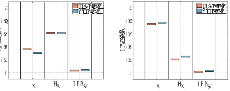
Figure 2. Main and total effects for η_E (left) and ΔV_c (right).

400 800 1200 1600 2000

No of model evaluations 0

0.1 0.2 0.3 0.4 0.5

Mean of EEs

R_{p p} SOC

in

400 800 1200 1600 2000

No of model evaluations 0

0.05 0.1 0.15 0.2 0.25 0.3

Mean of EEs

_p R p SOC_in

Figure 3. Convergence of the EEs for different numbers of model evaluations with 95% confidence intervals in the case ofη_E (left) and ΔV_c (right).

reaction rate depends upon the concentration (per unit volume of the electrode) of Li+according to the Butler-Volmer law (12), so a restricted supply of Li+in the positive electrode will lead to a large concentration overpotential for a fixed current (the overpotential in (12) must increase as

cdecreases in order to maintain a fixed left hand side, i.e, applied current density). The particle radius determines the level of mass transport resistance for the solid Li (which has to diffuse through the particle to react atR=R_p) as well as the specific surface area for reaction (smaller particles lead to higher specific areas). Thus, increasing the particle radius will lead to a higher concentration overpotential and, therefore, a deterioration in performance. For the voltage drop during discharge (ΔV_c),_phas the greatest influence, followed byR_p and lastly SOC_in, as seen in Figure 2. The combination of an increased Ohmic drop and a higher concentration overpotential on the total polarization caused by a lower _p outweighs the effect of an increased concentration overpotential caused by lowering R_p.

For an EET, uniform distributions were selected for the three factors, which were again scaled to yield X = [0,1]3. A major difference between the variance-based method and the EET is the sampling strategy. The EET is highly efficient, requiring only M(k + 1) model evaluations vs. N(k + 2) to calculate the main effect indices; in the results above,

N(k+ 2) = 5000×(3 + 2) = 25000, which is much higher than typical values of M(k+ 1). The trends in the means of the μ_i with confidence intervals (CIs) are depicted in Figure 3 for an increasing number of model evaluations (M(k+ 1)). The CIs were established using bootstrapping [14], which consists of re-sampling the base points with replacement to produce

P copies of the trajectories and for each of theP copies to use the EET to estimateμ_i and σ_i. This provides empirical distributions over μ_i and σ_i from which means and confidence bounds can be estimated.

p Rp SOCin

0 0.2 0.4 0.6 0.8 1

Sensitivity

1st coefficient

main effects total effects

p Rp SOCin

0 0.2 0.4 0.6 0.8 1

Sensitivity

2nd coefficient

main effects total effects

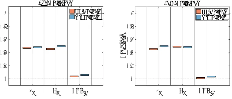
Figure 4. Main and total effects for the first two PCA coefficients (for the cell voltage curve).

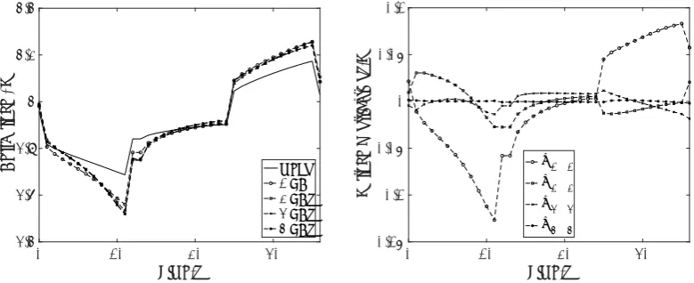
is used the much lower number of model runs for the EET represents an enormous advantage. To investigate the sensitivity of the charge-discharge curve, we examine the main and total effects of the PCA coefficientsw_i(ξξξ) using the same Latin hypercube design and N = 5000 (we replace, e.g.,η_E withw_i(ξξξ),i∈ {1, . . . , r}). The results are depicted in Figure 4 forw₁ and w₂. Figure 5 shows an example (from the test set) of the contributions from the PCA eigenvectors (w_iv_i, up toi= 4) towards the final (mean centred) voltage profile. The first two contributions can be seen to have by far the most influence. The sensitivities of the coefficientsw₁ and w₂ are highest for_pandR_p, with roughly equal contributions from each, while higher-order coefficients (w₃ and w₄) were more heavily influenced by SOC_in.

6. Summary and conclusions

SA is often unfeasible with complex computer models. In such cases emulators, of varying degrees of sophistication, can be employed. Quantifying the uncertainty in the emulator predictions is desirable, but this is only achievable for certain approaches. For multivariate outputs (especially in high dimensional spaces), SA under uncertainty is especially challenging, even when the QoI is a scalar. In this paper we propose a GP emulator approach for performing SA under uncertainty when the model output is multivariate (possibly in a high-dimensional space). We present an example for a Li-ion battery, demonstrating that the method can be efficient and accurate. We are able to perform a probabilistic SA on scalar QoIs derived from the output (via a linear functional) and also on the output itself by focusing individually on each random principal coefficient. This can be achieved with either full MC sampling or by using semi-analytical expressions that are extensions of those derived by Oakley and O’Hagan [5] for scalar QoIs.

0 10 20 30

Time/s 3.4

3.6 3.8 4 4.2 4.4

Cell voltage / V mean

1 PC 2 PCs 3 PCs 4 PCs

0 10 20 30

Time/s -0.15

-0.1 -0.05 0 0.05 0.1

Voltage contributions/V

w₁ v₁

w 2 v2 w

3 v3 w

4 v4

Figure 5. An example of the contributions from the PCA eigenvectors (w_iv_i) towards the final (mean centred) voltage profile. In the left-hand figure,w_iv_i is successively added to the mean.

References

[1] A. Saltelli, M. Ratto, T. Andres, F. Campolongo, J. Cariboni, D. Gatelli, M. Saisana, and S. Tarantola,

Global sensitivity analysis: the primer. John Wiley & Sons, 2008.

[2] D. Zhou, K. Zhang, A. Ravey, F. Gao, and A. Miraoui, Parameter sensitivity analysis for fractional-order modeling of lithium-ion batteries,Energies, 9, 123, 2016.

[3] M. D. Morris, Factorial sampling plans for preliminary computational experiments,Technometrics, 33, 161– 174, 1991.

[4] I. M. Sobol, Sensitivity estimates for nonlinear mathematical models,MMCE, 1, 407–414, 1993.

[5] J. E. Oakley and A. O’Hagan, Probabilistic sensitivity analysis of complex models: a Bayesian approach,R. Stat. Soc. Ser. B Stat. Methodol., 66, 751–769, 2004.

[7] A. Saltelli and I. M. Sobol’, Sensitivity analysis for nonlinear mathematical models: numerical experience,

Matematicheskoe Modelirovanie, 7, 16–28, 1995.

[8] I. Jolliffe,Principal Component Analysis. Springer Series in Statistics, Springer, 2002.

[9] D. Higdon, J. Gattiker, B. Williamsa, and M. Rightley, Computer model calibration using high-dimensional output,J Am. Stat. Assoc., 103, 570–583, 2008.

[10] C. Rasmussen and C. Williams, Gaussian Processes for Machine Learning. MIT Press, Cambridge MA, USA, 2006.

[11] M. Doyle, J. Newman, A. S. Gozdz, C. N. Schmutz, and J.-M. Tarascon, Comparison of modeling predictions with experimental data from plastic lithium ion cells,J. Electrochem. Soc., 143, 1890–1903, 1996. [12] https://www.comsol.

com/model/1d-lithium-ion-battery-model-for-internal-resistance-and-voltage-loss-determinat-19131, Last accessed 20 November 2017.

[13] F. Pianosi, F. Sarrazin, and T. Wagener, A matlab toolbox for global sensitivity analysis,Environ. Model. Softw., 70, 80–85, 2015.

[14] B. Efron, Bootstrap methods: Another look at the jackknife,Ann. Statist., 7, 1–26, 01 1979.

Appendix A. Efficient sampling for sensitivity analysis under uncertainty

We consider a scalar linear functional QoI Q= F(ξξξ) = (G◦η)(ξξξ) as defined in section 2. For example, we may considerG(y) =_Rη(x;ξξξ)w(x)dμ(x), for some measureμon a compact subset RofRLrepresenting space or time. To keep matters simple, we setw(x)≡1/μ(R), use Lebesgue measure and assume thatη(x;ξξξ) is continuous; then the Riemann and Lebesgue integrals coincide and approximations to G(y) by Riemann sums or Gauss quadratures converge. In reality of course we have a discrete output y_r = (y₁, . . . , y_d)T _=ηηη

r(ξξξ) that approximates η(x;ξξξ) at, say,

points {x_l}d_l=1 ⊂ R. Correspondingly, we have a discrete approximation g(y) of G(y) defined by a quadrature g(y_r) =μ(R)−1d_j=1b_jy_lj, where {y_lj}d_j=1 ⊂ {y_l}d_l=1 (approximating η(x_lj;ξξξ),

j= 1, . . . , d) is a subset of the coefficients of y_r and b_j are quadrature weights. If we are using a Gauss quadrature, the pointsx_lj are specified and must be included in the design{x_l}d_l=1. For ease of presentation, and without loss of generality, we use a mid-point Riemann sum, so that

f(ξξξ) =g(ηηη_r(ξξξ)) =g(y_r) =d−1d_l=1y_l.

Rather than a point estimate of y_r we have a distribution over functions (7), which leads to distributions over q = f(ξξξ) and therefore over the sensitivity measures, as a consequence of the emulator uncertainty. The typical sensitivity measures employed are S_i = V_i/V =

Var_ξi(E_ξξξ∼i[q|ξ_i])/Var(q) and S_Ti = 1−Var_ξξξ∼i(E_ξi[q|ξξξ_∼i])/Var(q). Oakley and O’Hagan [5] also propose the main effects f_i =E_ξξξ∼i[q|ξ_i]−f₀ as useful graphical summaries of the influences of each variable. We derive approximate estimates of the means and variances of these various quantities, extending the analysis in [5] to multiple output problems. Recalling relationship (7), namely,y_r =r_i=1w_i(ξξξ)v_i, and denoting the l-th component ofv_j by v_jl, we obtain:

Eηηηr

Eξξξ∼i[q|ξi]

=Eηηη_r

Eξξξ∼i 1 d d l=1

y_lξ_i

= 1

dEηηηr

⎡ ⎣_Eξξξ∼i

⎡ ⎣d

l=1 r

j=1

w_j(ξξξ)v_jlξ_i

⎤ ⎦ ⎤ ⎦

= 1

dEηηηr

⎡ ⎣_Eξξξ

∼i ⎡ ⎣r

j=1

b_jw_j(ξξξ)ξ_i

⎤ ⎦ ⎤ ⎦= 1

dEξξξ∼i

⎡ ⎣r

j=1

b_jEηηη_r[w_j(ξξξ)]ξ_i

⎤ ⎦

= 1

dEξξξ∼i

⎡ ⎣r

j=1

b_jm_j(ξξξ)ξ_i

⎤ ⎦= 1

d r j=1 b_j

[0,1]k−1

m_j(ξξξ)dξξξ_∼i= 1

d

r

j=1

b_jT_j(ξ_i)

(A.1)

whereb_j =d_l=1v_jland the functionsT_j(ξ_i) are defined by the integrals in the last line. Similarly:

Eηηηr[E[q]] = (1/d)

r

j=1

b_j

[0,1]k

m_j(ξξξ)dξξξ= (1/d)

r

j=1

where T_j are now constants since the integration is over all input factors. Thus Eηηη_r[f_i] =

Eηηηr[Eξξξ∼i[q|ξi]]−Eηηηr[E[q]] = (1/d) _r

j=1bj(Tj(ξi)−Tj). The integrals definingTj andTj can be

approximated numerically at a very low computational cost.

We denote by ξξξ_∼I the vector of factors excluding those corresponding to the index set I ⊂ {1, . . . , k} and denote byξξξ_I the subset of factors corresponding to I. From the definition of covariance we have:

Cov_ηηηrE_ξξξ∼I[q|ξξξ_I],E_ξξξ∼J[q|ξξξ_J]

=E_ηηηrE_ξξξ∼I[q|ξξξ_I]E_ξξξ∼J[q|ξξξ_J]−E_ηηηrE_ξξξ∼i[q|ξξξ_I]E_ηηηrE_ξξξ∼J[q|ξξξ_J]

=

ξξξ_∼J

ξξξ∼I

Eηηηr

f(ξξξ)f(ξξξ)dξξξ_∼Idξξξ_∼J −E_ηηηrE_ξξξ∼I[q|ξξξ_I]E_ηηηrE_ξξξ∼J[q|ξξξ_J]

=

ξξξ_∼J

ξξξ∼I

Cov_ηηηrf(ξξξ), f(ξξξ) −E_ηηηr[f(ξξξ)]E_ηηηrf(ξξξ)dξξξ_∼Idξξξ_∼J

−Eηηηr

Eξξξ∼I[q|ξξξI]

Eηηηr

Eξξξ∼J[q|ξξξJ]

=

ξξξ_∼J

ξξξ∼I

Cov_ηηηrf(ξξξ), f(ξξξ) dξξξ_∼Idξξξ_∼J

=

ξξξ_∼J

ξξξ∼I r j=1 r p=1

b_jb_pCov_ηηηrw_j(ξξξ), w_p(ξξξ) dξξξ_∼Idξξξ_∼J

= 1

d2

ξξξ_∼J

ξξξ∼I

r

j=1

b2_jc_j(ξξξ, ξξξ)dξξξ_∼Idξξξ_∼J =U(ξξξ_I, ξξξ_J)

(A.3)

in which the last step follows from the mutual independence of the w_i, and the

posterior covariances c_j(ξξξ, ξξξ) are given in Eqs. (6). Now, Var_ηηηr(f_i) = Eηηη_r[E_ξξξ2

∼i[q|ξi]] − 2E_ηηηr[E_ξξξ∼i[q|ξ_i]E[q]]−E_ηηηr[E2[q]]−E2_ηηηr[f_i] in which the last term on the right hand side is already known. The first to third terms are calculated by using the definition of covariance and Eq. (A.3) with (I,J) = ({i},{i}), ({i},∅) and (∅,∅), together with the previous expressions for

Eηηηr

Eξξξ∼i[q|ξi]

and Eηηη_r[E[q]]. The integrals in Eq. (A.3) are again cheap to evaluate. The means of all thef_i, evaluated separately for selected values of ξ_i in [0,1], can be combined on a single plot together with standard deviations to measure the influences of the factors [5] .

We next consider the partial variancesV_i. We first note thatEηηη_r[V_i] =Eηηη_r[Var_ξi(E_ξξξ∼i[q|ξ_i])] =

Eηηηr[Eξi[Eξξξ2∼i[q|ξi]]−E2ξi[Eξξξ∼i[q|ξi]]] =Eηηηr[Eξi[Eξξξ2∼i[q|ξi]]]−Eηηηr[E2[q]], the second term of which is already known. The first term is evaluated as follows:

Eηηηr

Eξi[Eξξξ2∼i[q|ξi]]

=Eηηη_r

[0,1]

[0,1]k−1f(ξξξ

∗_)dξξξ∗ ∼i

[0,1]k−1f(ξξξ)dξξξ∼i

dξ_i

=

[0,1]

[0,1]k−1

[0,1]k−1

Eηηηr[f(ξξξ)f(ξξξ∗)]dξξξ∗∼idξξξ∼idξi

=

[0,1]

[0,1]k−1

[0,1]k−1

{Cov_ηηηr(f(ξξξ), f(ξξξ∗))−E_ηηηr[f(ξξξ)]E_ηηηr[f(ξξξ∗)]}dξξξ∗_∼idξξξ_∼idξ_i

= 1 d2 r j=1

[0,1]

[0,1]k−1

[0,1]k−1bj

⎧ ⎨

⎩bjcj(ξξξ, ξξξ∗)− r

p=1

b_pw_j(ξξξ)w_p(ξξξ∗) ⎫ ⎬

⎭dξξξ∗∼idξξξ∼idξi

(A.4)