Multi objective new product development by complete Pareto front and ripple spreading algorithm

http://wrap.warwick.ac.uk/

Hu, Xiao-Bing, Wang, Ming, Ye, Qian, Han, Zhangan and Leeson, Mark S., 1963-. (2014) Multi-objective new product development by complete Pareto front and ripple-spreading algorithm. Neurocomputing , Volume 142 . pp. 4-15.

Permanent WRAP url:

http://wrap.warwick.ac.uk/63879

Copyright and reuse:

The Warwick Research Archive Portal (WRAP) makes this work of researchers of the University of Warwick available open access under the following conditions. Copyright © and all moral rights to the version of the paper presented here belong to the individual author(s) and/or other copyright owners. To the extent reasonable and practicable the material made available in WRAP has been checked for eligibility before being made available.

Copies of full items can be used for personal research or study, educational, or not-for-profit purposes without prior permission or charge. Provided that the authors, title and full bibliographic details are credited, a hyperlink and/or URL is given for the original metadata page and the content is not changed in any way.

Publisher statement:

NOTICE: this is the author’s version of a work that was accepted for publication in Neurocomputing. The changes resulting from the publishing process, such as peer review, editing, corrections, structural formatting, and other quality control mechanisms may not be reflected in this document. Changes may have been made to this work since it was submitted for publication. A definitive version was subsequently published in

http://dx.doi.org/10.1016/j.neucom.2014.02.058

A note on versions:

The version presented here may differ from the published version or, version of record, if you wish to cite this item you are advised to consult the publisher’s version. Please see the ‘permanent WRAP url’ above for details on accessing the published version and note that access may require a subscription.

Multi-Objective New Product Development by

Complete Pareto Front and Ripple-Spreading

Algorithm*

Xiao-Bing Hu

, Ming Wang

, Qian Ye

, Zhangang Han

, and Mark S. Leeson

1

State Key Laboratory of Earth Surface Processes and Resource Ecology,

Beijing Normal University, China.

2

School of Systems Science, Beijing Normal University, China.

3

School of Engineering, University of Warwick, Coventry, UK.

* _{This work was supported in part by the China “973” Project under Grant 2012CB955404, the project grant 2012-TDZY-21}

Abstract

Given several different new product development projects and limited resources, this paper is concerned

with the optimal allocation of resources among the projects. This is clearly a multi-objective optimization

problem (MOOP), because each new product development project has both a profit expectation and a loss

expectation, and such expectations vary according to allocated resources. In such a case, the goal of

multi-objective new product development (MONPD) is to maximize the profit expectation while

minimizing the loss expectation. As is well known, Pareto optimality and the Pareto front are extremely

important to resolve MOOPs. Unlike many other MOOP methods which provide only a single Pareto

optimal solution or an approximation of the Pareto front, this paper reports a novel method to calculate the

complete Pareto front for the MONPD. Some theoretical conditions and a ripple-spreading algorithm

together play a crucial role in finding the complete Pareto front for the MONPD. Simulation results

illustrate that the reported method, by calculating the complete Pareto front, can provide the best support to

decision makers in the MONPD.

Key words: Multi-Objective Optimization, New Product Development, Pareto Front, Ripple-Spreading

Algorithm.

1 INTRODUCTION

New product development plays an extremely crucial role in company survival and success in the

modern increasingly competitive global market; every year, billions of dollars are invested in various new

product development projects (NPDPs) worldwide [1]-[5]. Obviously, not all NPDPs are successful, and

there never lack examples where a big-brand company collapses after an NPDP because it misjudges

market trends and/or consumes considerable of capital. To avoid such a tragedy, an effective practice is

"not to put all eggs in one basket". Therefore, a company may often have several NPDPs proceeding at one

time. Each NPDP has both a profit expectation and a loss expectation, and such expectations vary

according to the resources allocated to the NPDP. Basically, the greater the allocated resources the higher

the profit expectation is. Increased allocated resources may reduce the failure possibility during the

development stage of an NPDP, but cannot necessarily provide a better guarantee of market success. If

anything goes wrong during the marketing stage due to many external, uncertain and uncontrollable factors,

the larger resource allocation only means a bigger loss. Common sense in the financial sector predicts that

have to make a choice between high-profit-big-risk options and low-profit-small-risk options, based on

their risk taking willingness and understanding of a market environment. Since available resources are

always limited, decision makers usually need to optimize their investment portfolio, in order to maximize

the profit expectation while minimizing the loss expectation – two conflicting objectives. In this paper, we

are particularly concerned with the problem of allocating limited resources among several NPDPs, so that

the overall profit expectation can be maximized while the overall loss expectation can be minimized. This

clearly fits in the scope of a multi-objective optimization problem (MOOP), and hereafter we call the

concerned problem multi-objective new product development (MONPD).

To resolve the MONPD, we need to make use of the Pareto front. As the most important concept in

MOOPs, the Pareto front originates from the concept of Pareto efficiency proposed to study economic

efficiency and income distribution [7]. In general MOOPs, a solution is called Pareto optimal if there

exists no other solution that is better in terms of at least one objective and is not worse in terms of all other

objectives [8] [9]. The projection of a Pareto optimal solution in the objective space is called a Pareto point.

All Pareto points, i.e., the projections of all Pareto optimal solutions, compose the complete Pareto front of

an MOOP.

The history of such problems is long resulting in the development of many methods for resolving

various MOOPs. Basically, most methods can be classified into three categories: aggregate objective

function (AOF) based methods [10]-[14], Pareto-compliant ranking (PCR) based methods [15]-[25], and

constrained objective (COF) function based methods [26]-[30]. An AOF method combines all of the

objectives of an MOOP to construct a single aggregate objective function, and then resolve the

single-objective problem to get a Pareto optimal solution. However, it involves subjectiveness in

constructing an AOF, and it often fails to find some Pareto optimal solutions if the Pareto front is not

convex. A PCR method may overcome such drawbacks of AOF methods by operating on a pool of

candidate solutions and favoring non-dominated solutions. Population-based evolutionary approaches

(such as genetic algorithms, particle swarm optimization and ant colony optimization) often play a key role

in PCR methods to identify multiple Pareto optimal candidate solutions. It should be noted that, due to the

stochastic nature of PCR methods, their outputs are Pareto optimal candidate solutions, not necessarily

real Pareto optimal solutions. Theoretically, COF methods, by optimizing only one single objective while

treating all other objectives as extra constraints, may avoid both the subjectiveness of AOF methods and

the loss of Pareto optimality in PCR methods.

Calculating complete Pareto front is a relatively less discussed topic in the study of MOOPs.

a set of AOF coefficients definitely exists which can lead to that Pareto point. However, the difficulty is

that there a lack of a practicable method to find those sets of coefficients that will help to identify the

complete Pareto front [28]. For PCR methods, guaranteeing the complete Pareto front is theoretically a

mission impossible, largely because of the stochastic nature of employed population-based approaches

[15]. COF methods, given well posed objective function constraints, may theoretically guarantee the

finding of the complete Pareto front but like AOF methods, how the practicality of finding proper

constraints is a big issue [30]. Therefore, most existing methods can only produce an incomplete or

approximate Pareto front [10], [15], [26]-[30]. In particular, as pointed out in [26], very few results are

available on the quality of the approximation of the Pareto front for discrete MOOPs.

We have recently proposed a deterministic method which can, theoretically and practically, guarantee

the finding of complete Pareto front for discrete MOOPs [31]. Some theoretical conditions and a general

methodology were reported in [31], and a case study on a multi-objective route optimization problem

(ROP) was used to prove the correctness and practicability. In this paper, we will particularly apply the

method of [31] to the MONPD. Actually, there is a substantial body of literature on optimizing investment

portfolios [6], [32]-[38] similar to MONPD, but little work has been reported to calculate complete Pareto

front of such investment portfolio optimization problems. To calculate the complete Pareto front for

MONPD, firstly, we will improve the theoretical conditions and the methodology reported in [31]. The

most challenging part in the method of [31] is to design an algorithm that is capable of finding the global

kth best solution for any given k in terms of a given single objective. Designing such an algorithm is largely

problem-dependent, and is often difficult because most optimization algorithms only calculate the global

1st best solution. MONPD is quite different from the ROP in [31]. For example, in the ROP, every

objective needs to be minimized; however, in MONPD, the profit expectation needs to be maximized

although the loss expectation is to be minimized. Therefore, MONPD demands a new algorithm to

calculate the general kth best (rather than only the kth smallest) single-objective solution. By successfully

developing a new ripple-spreading algorithm for MONPD, this paper will further prove the practicability

and the potential of the methodology of resolving discrete MOOPs by calculating complete Pareto front.

The remainder of this paper is organized as following. Section 2 gives some theoretical results for

calculating complete Pareto front for discrete MOOPs. Section 3 describes mathematically the details of

MONPD. Section 4 reports a ripple-spreading algorithm for MONPD. Simulation results are given in

2 THEORETICAL RESULTS FOR CALCULATING THE COMPLETE PARETO FRONT

We have recently reported some theoretical results and a general methodology to guarantee,

theoretically and practicably, the finding of the complete Pareto front for discrete MOOPs [31]. The work

in [31] is the theoretical foundation of this application paper. In this section, we will introduce some

improvements to the work of [31], in order to better apply to MONPD later.

First of all, we need a general mathematical formulation of discrete MOOPs as following:

_N T

x

x g x g x g

Obj( )]

),..., ( ), ( [

min

subject to

h_I( x)≤0, (2)

0

=

) ( x

h_E , (3)

X

x∈Ω , (4)

where gi is the ith objective function of the total NObj objective functions, hI and hE are the inequality and

equality constraints, respectively, x is the vector of optimization or decision variables belonging to the set

of Ω_X, and x is of discrete value. A Pareto-optimal solution x* to the above problem is so that there exists

no x that makes

g_i(x)≤ g_i(x*), for all i=1,..,NObj, (5)

g_j(x)< g_j(x*), for at least one j ∈[1,..,N_Obj]. (6)

The projection of such an x* in the objective space is called a Pareto point. The above problem usually has

a set of Pareto optimal solutions, whose projections compose the complete Pareto front.

2.1Theoretical conditions

According to the theoretical results in [31], we have the following statements for discrete MOOPs.

Lemma 1: Suppose we sort all discrete x∈Ω_X according to a certain objective function gj(x), and xj,i

has the ith smallest gj. For a given constant c, if there exists an index k that satisfies

gj(xj,k)≤c< gj(xj,k+1), (7)

Then the number of Pareto points whose gj≤c is no more than k, and all the associated x values are included

in the set [xj,1,…,xj,k].

Lemma 2: Suppose we have a constant vector [ ,..., ]

Obj

N c

c₁ , the element cj is for objective function gj,

and after sorting all discrete x∈ΩX according to each objective function gj, we have kj satisfying

( _, ) ( _, ) i

j i ik

k j

i x g x

g ≤ , for all i≠j, (8)

then the total number of Pareto points is no more than

∑

, (9)

and all associated x values are included in the union set

U

U x x

1

, 1 ,

1 [ ,..., ]

=

=

Ω , j=1,…,NObj. (10)

For more details about Lemma 1 and Lemma 2, one may refer to [31]. Based on Lemma 1 and Lemma

2, [31] reported a methodology which employs an iteration process to calculate the kj best solutions in

terms of objective function gj, for all j=1,…,NObj. In the iteration process, kj is increased step by step for all

j=1,…,NObj, until a set of [k1,...,kNObj] is found to make Condition (8) hold.

In this paper, we give an upper bound for kj (or upper bound for cj), j=1,…,NObj, in order to improve the

computational efficiency of the methodology in [31]. To this end, we need the following new theorems.

Theorem 1: Suppose there exist

Obj

N x

x ,...,₁ such that for any j∈[1,...,NObj],

g_i(x_j)≤ g_i(x_i), for all i=1,..,NObj. (11)

Then all Pareto-optimal solutions are included in the union set

)} ( ) ( : { 1

2 i i i

N

i

U x g x g x

Obj

≤ =

Ω

=

U _{. (12)}

Proof: Assume Theorem 1 is false. Therefore, there exists at least one Pareto-optimal solution, say x*,

that does not belong to the union set Ω_U2, which means, according to the definition of Ω_U2 in Eq.(8), we

have g_i(x_i)< g_i(x*) for all i=1,..,NObj. Then for any j∈[1,...,NObj], we have

( ) ( ) ( *) x g x g x

g_{i j} ≤ _{i i} < _i , for all i=1,..,NObj. (13)

This means

Obj

N x

x ,...,₁ are all more Pareto efficient than x*. In other words, x* is not a Pareto-optimal

solution at all. Therefore, the assumption must be false, and Theorem 1 must be true.

Corollary 1: Obviously, the set of the first best single-objective solutions [ _1,1,..., _,1] Obj

N x

x satisfies

Condition (11) in Theorem 1. Therefore, all Pareto-optimal solutions are included in the union set

)}

(

)

(

:

{

1

3 i i i

N

i

U

x

g

x

g

x

Obj

≤

=

Ω

=

U

With the union set defined by Eq.(14), we have

Theorem 2: The constant vector [ ,..., ]

Obj

N c

c₁ in Lemma 2 has an upper bound defined by

) ( ,1 ,...,

1

max

N i

j g x

c

Obj =

= , j=1,…,NObj. (15)

Suppose the cj in Eq.(15) is the (kj)

th

for kj in Lemma 2, j=1,…,NObj.

Proof: Assume Theorem 2 is false, i.e., for at least a j∈[1,...,N_Obj], there exists no c_j≤cj that can

make Condition (8) hold. This means that the complete Pareto front is not covered by the union set Ω_U1, in

other words, there exists at least one Pareto-optimal solution x* that has c_j < g_j(x*). Then according to

Eq.(14) and Eq.(15), one has that this x* is not included in the union set Ω_U3, which is obviously against

Corollary 1. Therefore, Theorem 2 must be true.

2.2General methodology

In this sub-section, based on Theorem 1 and Theorem 2, we will modify the methodology reported in

[31], in order to improve the computational efficiency. The modified general methodology to calculate the

complete Pareto front for discrete MOOPs is described as following:

Step 1. Design a problem-dependent deterministic algorithm that is capable of calculating any global kth

best solution in terms of a single objective function gj, for any j=1,…,NObj.

Step 2. Calculate the set of the first best single-objective solutions [ _1,1,..., _,1] Obj

N x

x , and then determine

the upper bound set [ ₁,..., ] Obj

N c

c according to Eq.(15).

Step 3. Initialize kj=1, for every j=1,…,NObj. Initialize the Pareto front associated x value set as

∅ =

ΩPFX . Calculate the (kj+1)th global best solutions in terms of the single objective function gj,

i.e., calculate _{, +1} j

k j

x , for every j=1,…,NObj.

Step 4. If for every j=1,…,NObj,

( _, )< ( _{, +1})

j

j j jk

k j

j x g x

g , (16)

( _, ) ( _, )

i

j i ik

k j

i x g x

g ≤ , for all i≠j, (17)

then go to Step 6. Otherwise, fix kj for any j that has Conditions (16) and (17) both satisfied or has

j k j

j x c

g

j)≥

( _, , and increase kj by one, i.e., kj=kj+1, for the j that has Condition (16) satisfied for the

most i values.

Step 5. For the newly increased kj, calculate the (kj+1)th global best solutions in terms of gj, i.e., update

1 ,kj+

j

x . Go to Step 4.

Step 6. Calculate the union set of [ _,1,..., _, ] j

k j

j x

x , j=1,…,NObj, denoting as ΩUX.

Step 7. For any x∈ΩUX, if there exist no x∈ΩUX

(

such that gi(x)≤gi(x)

(

, for all i=1,..,NObj, and

) ( )

(x g x

g_j ( < _j , for at least one j ∈[1,..,N_Obj], then we know the point [ ,..., ]

Obj

N

g

g₁ is a Pareto point.

The basic methodology in [31] needs to keep calculating the k best solutions in terms of each

single-objective function in the iteration process, whilst the modified methodology only calculates the kth

best single-objective solution in Step 2, Step 3 and Step 5. Another improvement in the modified

methodology is the introduction of upper bound c in Step 4, which avoids unnecessary operation of _j

increasing any kj with gj(xj,kj)≥ cj. These modifications may obviously improve the computational

efficiency to find the complete Pareto front for a discrete MOOP.

3A MATHEMATICAL FORMULATION OF MONPD

Basically, MONPD is to allocate limited resources among several different new product development

project (NPDPs), in order to maximize the profit expectation and minimize the loss expectation. Here we

give a mathematical description of the MONPD as following, which is illustrated by Fig.1.

Fig.1. Illustration of MONPD

Suppose we have limited resources, X , to support NP NPDPs. Let x denote an allocation strategy, and

0≤x(i)≤X denote the resources allocated to NPDP i, for i=1,...,NP. With allocated resources x(i), the profit

expectation of NPDP i is g1,i(x(i)), and the associated loss expectation is g2,i(x(i)). Then for an allocation

strategy x, the total profit expectation and loss expectation are

∑

=

=

i

i

x

i

g

g

1 , 1

∑

=

=

i

i

x

i

g

g

1 , 2

2

(

(

))

respectively. Then, with g1 and g2 as two objective functions, MONPD is formulated as

1

max

g

x

, and

min

g

x

(20)

subject to (18), (19) and

∑

=

=

i

i

x

X

1

)

(

The work in [31] is used to calculate complete Pareto front for discrete MOOPs. In this study, we

assume there is a minimal investment unit ∆x for resource allocation, and for any i=1,...,NP, we have

x

(

i

)

=

n

(

i

)

∆

x

X

=

N

∆

x

then we know for each i=1,...,NP, x(i) has (NTNIU+1) choices, i.e.,

x

(

i

)

∈

{

0

,

∆

x

,...,

N

∆

x

}

the minimal investment unit ∆x, Constraint (21) is equivalent to

∑

=

=

i TNIU

n

i

N

1

)

(

(a) Contribution curves to g1 (b) Contribution curves to g2 Fig.2. Illustration of contribution curves

i with allocated resources x(i) to objective function gj, i=1,...,NP, and j=1,2. Basically, a contribution curve

is nonlinear, and the MONPD involves a combination of different shaped nonlinear contribution curves.

The complexity is illustrated by the contribution curves in Fig.2, where there are 3 NPDPs, and therefore 6

contribution curves of different shapes, which are totally project-dependent. Regarding the profit

expectation of NPDP i, there is usually a threshold xT,i, and if the allocated resources to NPDP i is below

the threshold, i.e., x(i)≤xT,i, then the project has no way to succeed, and therefore will make no profit at all.

Regarding the loss expectation of NPDP i, when x(i)≤xT,i, the loss often linearly increases as x(i) goes up,

and the gradient largely depends on what percentage of x(i) is invested in reusable facilities.

Fig.3. Complete Pareto front and approximations

For discrete MONPD, a typical complete Pareto front is given in Fig.3, which is composed of squares

and solid lines. Since the MONPD needs to maximize g1 and minimize g2 simultaneously, the Pareto front

is an increasing curve. It should be noted that the Pareto front of the ROP in [31] is a decreasing curve,

because all objectives need to be minimized there. Therefore, as will be explained later in Section 4.2, the

method design for MONPD is rather different from that for the ROP in [31]. Such an increasing curve in

MONPD implies a large profit expectation always comes with a large loss expectation. Any point in the

right-bottom side of the Pareto front is impossible to achieve. For any point in the left-top side of the

Pareto front, the associated x is not Pareto optimal, which means there exists at least one solution leading

to a larger profit expectation without increasing the loss expectation, or a smaller loss expectation without

decreasing the profit expectation. Fig.3 also gives two approximations of the Pareto front and one is

plotted by circles and dash-and-dot lines, and the other by triangles and dash lines. As illustrated in Fig.3,

usually uncertain to decision makers, in other words, if an approximation of the Pareto front is provided,

decision makers will have no idea whether there exists any other Pareto-optimal solution (e.g., in Fig.3,

Approximation 2 misses out one Pareto point, which is probably the best tradeoff between two objectives),

or even whether a provided solution associated with a point on the approximated Pareto front is really

Pareto-optimal (e.g., in Fig.3, Approximation 1 actually has 3 false Pareto points). Therefore, using an

approximation of Pareto front implies (i) some solutions most preferable by decision makers might be

actually missed out, and (ii) arguments might occur in the decision making process because different

decision makers could choose different approximation methods. Obviously, if we can calculate the

complete Pareto front rather than approximating it, then decision makers will be free of the above issues.

With the complete Pareto front at hand as illustrated in Fig.3, decision makers in MONPD can easily and

accurately find an ideal resource allocation strategy according to, say, their risk-taking willingness and

market uncertainties.

4 A RIPPLE-SPREADING ALGORITHM FOR MONPD

4.1 Basic idea of ripple-spreading algorithm (RSA)

It is well known that many successful computational intelligence techniques are actually inspired by

certain natural systems or phenomena [39]. For instance, genetic algorithms are inspired by natural

selection and evolutionary processes, artificial neural networks by the animal brain, particle swarm

optimization by the learning behavior within a population, and ant colony optimization by the foraging

behavior of ants. Following the common practice of learning from nature in the computational intelligence

domain, we have recently reported some ripple-spreading models and algorithms [40]-[44]. The

hypothesis behind these is the following: the natural ripple-spreading phenomenon, as a pervasive

phenomenon in the universe, reflects certain fundamental organization/optimization principles in nature,

and such principles are to be found in many systems and problems around us. Taking such inspiration

when developing models and algorithms to study such systems and problems, we are likely to better

match/reflect the embedded principles of these systems, and therefore generate more effective solutions.

For example, by mimicking the natural ripple-spreading phenomenon, we developed some useful models

to study complex networks [40], air traffic management [41], and epidemic dynamics [42], and some

effective algorithms to tackle ROPs [43], [44].

Basically, ripple-spreading algorithms (RSAs) achieve optimality by taking advantage of the

optimization principle reflected in the natural ripple-spreading phenomenon, which is very simple: a ripple

their distance from the ripple epicenter, i.e., it always reaches the closest point first. Intuitively, one may

get a feeling that this optimization principle could be used to find the closest interesting points (e.g., to find

the closest gas station), or more generally, to find the shortest path. Therefore, we successfully developed

some effective RSAs for ROPs in [43] and [44]. Most existing methods for ROPs are centralized,

top-down, logic-based search algorithm. Differently, RSAs are actually decentralized, bottom-up,

agent-based simulation model. By defining the behavior of individual nodes, optimality will automatically

emerge as a result of the collective performance of the model. As illustrated in Fig.4, the first ripple starts

from the source node, i.e., node 1; when a ripple reaches a directly connected but unvisited node, that new

node will be activated to generate its own ripple; when all of those nodes that are directly connected to the

epicenter node of a ripple are visited (not necessarily by the same ripple), that ripple will then stop and be

eliminated; when the destination node, i.e., node 4, is visited for the first time, the first shortest route is

then found [43]; the simulation keeps going on until the destination node is reached for the kth time, then

the k shortest routes are found in order [44]. The above process is likened to a ripple relay race, where

ripples compete with each other to reach the destination node. During the entire process, all ripples always

travel at the same preset constant speed.

4.2 Bespoke RSA for MONPD

The most difficult part of the general methodology in Section 2.2 is to find/design a problem-specific

algorithm to calculate the k best single-objective solutions to an MOOP. In this sub-section, we will design

an RSA which is capable of calculating the k best solutions in terms of the profit expectation g1 and the

loss expectation g2, respectively.

As discussed in Section 4.1, the RSA in [44] can resolve the k shortest paths problem. To apply a RSA

to the MONPD, we need to transform the MONPD into a special ROP. Please note that the ROP in [44] is

a minimization problem, whilst optimizing profit expectation is a maximization problem. Therefore, we

have to make some modifications before we can apply RSA to the MONPD.

To transform the MONPD into a ROP, we need to construct two directed route networks for the

MONPD, one for g1 and the other for g2. In the route network for gj, firstly we set up a dummy source node.

Then we add NTNIU+1 new nodes, representing different resource allocations to NPDP1. Then we establish

directed links from the source to each of these NTNIU+1 nodes. In the route network for g1, the length of the

link which connects to the node of n∆x allocation to NPDP1 is set as

l_n,1 = g_1,1(X)−g_1,1(n∆x), n=0,…, NTNIU, (25)

and in the route network for g2, the length is

ln,1 = g2,1(n∆x), n=0,…, NTNIU. (26)

Assume we have added NTNIU+1 nodes associated with different resource allocations to NPDP i, i<NP-1.

Then we add another NTNIU+1 new nodes, representing different resource allocations to NPDP i+1. Then

we establish directed links from NPDP i nodes to NPDP i+1 nodes subjected to Constraint (21) or (24). In

the route network for g1, the length of the link which connects to the node of n∆x allocation to NPDP i+1 (i.e., x(i+1)=n∆x) is set as

l_n,i+1 = g_1,i+1(X)−g_1,i+1(n∆x), n=0,…, NTNIU, (27)

and in the route network for g2, the length is

ln,i+1 = g2,i+1(n∆x), n=0,…, NTNIU. (28)

After we have added NTNIU+1 nodes associated with different resource allocations to NPDP NP-1, then we

add a dummy destination node, and establish a directed link from every NPDP NP-1 node to the destination.

As will be explained later, the length of a link connected to the destination, denoted as ln,NP, will be

dynamically set up during the following ripple relay race. Fig.5 gives a simple illustration about how to

With the constructed route network for gj, we can develop a ripple relay race to calculate the k best

solutions in terms of objective gj for MONPD. Basically, the new race process is similar to that in [44],

which aims to resolve the k shortest paths problem, and the major modifications are: (i) a new ripple at a

node needs to select out feasible links from established links according to Constraint (21) or (24); (ii) the

length ln,NP needs to be dynamically reset according to the resource allocations of NPDP1 to NPDP NP-1.

Since a ripple-spreading algorithm is actually a bottom-up, agent-based simulation model we can easily

define problem-specific node behavior to achieve the above two modifications. Therefore as a result of the

above two modifications, the route network for gj in MONPD can be viewed as a dynamic network rather

than the static ones in [31], [43] and [44].

Fig.5 The construction of route network for gj in MONPD

The following are the details of the new ripple relay race to calculate the k best solutions in terms of

objective gj for MONPD.

Step 1. Set the ripple spreading speed as s. Set time t=0. Let nDNR=0 denote how many times the dummy

destination node has been reached by ripples. Start an initial ripple at the dummy source node. In the

relay race, every ripple needs to record which existing ripple triggers it, and which node it originates.

For the initial ripple at the dummy source node, it is triggered by no other existing ripple.

Step 2. If nDNR<k, update t=t+1, and repeat the following process. For each existing ripple, increase its

radius by s. Compare its radius with the length of every feasible link. As emphasize before, the route

network of MONPD is a dynamic network. Although we have established a static network topology

all established links are feasible to travel on. Suppose a stimulating ripple passes the NPDP m node

of n(m)∆x, m=1,...,i-1, and then trigger a new ripple at the NPDP i node of n(i)∆x. Then, for this

new ripple, an established link connected to the NPDP i+1 node of n(i+1)∆x is feasible if

∑

X . (29)

The dynamic feature of the MONPD network also results from the length of a link from an NPDP

NP-1 node to the dummy destination node, which depends on the so-far route along which the

stimulating ripple of the current NPDP NP-1 ripple travels. Suppose the stimulating ripple passes the

NPDP i node of n(i)∆x, i=1,...,NP-2, and the current NPDP NP-1 ripple originates from the NPDP

NP-1 node of n(NP −1)∆x, then in the route network for g1, the link length from the NPDP NP-1

node of n(N_P −1)∆x to the dummy destination node is

( ) ( ( ) ) 1 1 , 1 , 1 ,

∑

= _{P P} P

P N i N N N

n g X g X n i x

l , (30)

and in the route network for g2, the link length is

( ( ) ) 1 1 , 2 ,

∑

= _P P

P

N

i N

N

n g X n i x

l . (31)

If the radius is larger than a feasible link,

Step 2.1. If the end node of the feasible link is not the dummy destination node, then a new ripple

will be triggered at the end node of the feasible link, and the initial radius of the new ripple is the

radius of the stimulating ripple minus the length of the feasible link.

Step 2.2. If the end node of the feasible link is the dummy destination node, then update nDNR=

nDNR+1. Track back the current ripple to reveal the (nDNR)th best solution in terms of objective gj.

If nDNR=k, go to Step 3.

Step 3. Stop the ripple relay race, and output the k best solutions in terms of objective gj.

It is easy to derive that the kth shortest path in the constructed route network for gj is associated with the

kth best solution in terms of optimizing the value of gj (i.e., maximizing g1 or minimizing g2). With the

above ripple-spreading algorithm, the methodology in Section 2.2 becomes practicable for MONPD. One

may argue that, for the sake of computational efficiency, the methodology in Section 2.2 demands an

algorithm to calculate the kth best single-objective solution rather than the k best single-objective solutions.

This is not a problem at all. When integrating the above ripple-spreading algorithm into the methodology

destination node is reached by a ripple, the race process will be paused or frozen. Then the newly found

best solution will be checked with all previously found best solutions, to see if the complete Pareto front is

covered. If not, then the race process will be resumed to find the next best solution.

The optimization of profit expectation g1 defined in (20) is a maximization problem, to which the RSA

in [26, [43] and [44] cannot apply directly. The setup of link length according to (25), (27) and (30) in

the route network for g1 actually converts the original maximization of g1 into a minimization problem.

This design enables the calculation of the kth largest profit expectation by the RSA. Similar to

approaches in [43] and [44], one may derive that the optimality of the RSA reported in this section is

guaranteed by the optimization principle reflected in the natural ripple-spreading phenomenon. In other

words, the reported RSA can theoretically guarantee the finding of the kth best single-objective solution

for MONPD. Therefore, applying the general methodology in Section 2.2 to calculate the complete

Pareto front of MONPD becomes practically possible.

5 SIMULATION RESULTS

In this section, we present some simulation results to demonstrate the practicability and effectiveness of

the proposed method to calculate the complete Pareto front for MONPD. There are three parts of

simulation results: (i) comparative results with a brute-force search (BFS) method to prove the discovery

of the complete Pareto front; (ii) comparative results with an aggregate objective function (AOF) based

method and a Pareto-compliant ranking (PCR) based method to show the advantage of new method; (iii)

analyses based on the complete Pareto front to illustrate the usefulness of the new method. In the

simulation, the total budget X has 9 options: [10 15 20 25 30 35 40 45 50] (million money unit), which

represent 8 scenarios. Resources need to be allocated to five different NPDPs, whose profit expectations

and loss expectations are given in Fig.6. Basically, the profit expectations all go up as the allocated

resources increase. For NPDP1 to NPDP4 (e.g., traditional categories of products such as clothes, toys and

food), the profit expectation will approach a certain upper bound gradually, while for NPDP5 (e.g.,

high-tech products such as online games), the profit expectation rises exponentially. Both expectation

curves of NPDP3 are piece-wise, and this is usually related to contracted order of customized product. In

other words, a new product is especially developed according to the order of a certain customer, and once

developed successfully, will be sold for sure (therefore the loss expectation may become zero once the

basic order is fulfilled), but only to that customer. Further development may be carried out beyond the

basic order, but the customer is not contracted to buy or pay a higher price. Therefore, the loss expectation

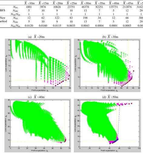
In the comparison with BFS, the minimal investment unit ∆x is set as 1 million, so that the simulation results can be better plotted to demonstrate the advantage of new method. Some results are given in Table

1 and Fig.7, where NNS is total number of solutions explored by a method, NPPF is number of Pareto points

found by a method, NSS is the total number of solutions in the solution space, and NNS/NSS indicates the

search efficiency of a method. Firstly, the simulation results confirm that the Pareto fronts identified by the

new method are exactly the same as those found by the BFS. Table 1 shows that the Pareto fronts found by

the new method have exactly the same number of Pareto points as those by the BFS. From Table 1, one can

also see the new method has a much better search efficiency than the BFS, and in general, the advantage

becomes more significant as the problem complexity increases (i.e., when X goes up). Fig.7 gives four

examples to illustrate why the new method is much more computationally efficient. According to the

theories in [31], the solutions explored by the new method are only those pink star points (including all

Pareto point plotted as red circles), which are below or on the right-hand side of the yellow dash lines in

Fig.7. Those yellow dash lines are drawn according to the kth best solutions which trigger the termination

criteria of the new method, i.e., Conditions (16) and (17) in Section2.2. For example, in the case of Fig.7(c),

the 7th best solution in terms of g1 and the 6th best solution in terms of g2 satisfy the Conditions (16) and

(17). Because of the ripple-spreading nature when searching for the kth best single-objective solution, the

new method simply stops before any more solution is explored. Those green star points in Fig.7 are all

solutions which are not explored by the new method. When comparing those green star points and those

pink ones, one may get an intuitive feeling how computationally efficient the new method could be against

the BFS.

Table 1 Comparative results between BFS and the new method (∆x is set as 1 million)

X=10m X=15m X=20m X=25m X=30m X=35m X=40m X=45m X=50m

BFS

NNS 1001 3876 10626 23751 46376 82251 135751 211876 316251

NPPF 5 10 9 10 13 7 5 12 29

NNS/NSS 1 1 1 1 1 1 1 1 1

New method

NNS 12 62 122 83 198 34 12 66 306

NPPF 5 10 9 10 13 7 5 12 29

NNS/NSS 0.0120 0.0160 0.0115 0.0035 0.0043 0.0004 0.0001 0.0003 0.001

(a) X=20m (b) X=30m

(c) X=40m (d) X=50m

Fig.7 Completeness of the calculated Pareto fronts (∆x is set as 1 million)

Now, we compare the new method with two of the most popular MOOP methods: one is an AOF

method, and the other is a well known PCR method, i.e., the NSGA-II in [19]. This time, we increase the

portfolio optimization [32], the two objective functions g1 and g2 are integrated as follows

gAOF =wg1+(1−w)g2, (32)

where 0≤w≤1 is a weight. In the simulation, for each scenario of MONPD, we change value of w from 0 to 1 with a step of 0.01. For each w value, we run the AOF method, and get a Pareto point. Then we use all

Pareto points generated by the AOF method to approximate the true Pareto front. In the simulation, the

NSGA-II has a population size of 100, a crossover probability of 0.5, a mutation probability of 0.1, and

evolves 200 generations. For each scenario of MONPD, the NSGA-II is run for 100 times. Fig.8 gives the

complete Pareto fronts found by the new method, and Table 2 gives the results of different methods, where

NPPF shows how many real Pareto points a method has found, NTPP is total number of real Pareto points in

a certain scenario, and PFCPF is the probability for a method to find the complete Pareto front. From Table

2, one can see clearly that: (i) the reported new method is the best, because it can always guarantee the

finding of the complete Pareto fronts for the MONPD; (ii) except in the scenario of X =40m (where the

Pareto front is convex), the AOF method cannot find any complete Pareto front, because those fronts are

not convex (see Fig.8); (iii) NSGA-II is better than the AOF method, but due to its stochastic nature,

NSGA-II cannot guarantee to find the complete Pareto front for the MONPD every time, in particular, the

probability of success drops significantly in complex scenarios such as X =45m and X =50m. Please note

that, during a run of the NSGA-II, a set of currently non-dominated solutions is developed, and it is the

final set of currently non-dominated solutions, not the last generation of chromosomes, that is used to

approximate the Pareto front. Therefore, in the case of X =50m, although the population size, i.e., 100, is

smaller than the total number of Pareto points, i.e., NTPP=176, the NSGA-II may still find the complete

Pareto front in some runs. However, when compared with the new method, the chance for the NSGA-II to

success is very poor in the case of X =50m. From Table 1, Table 2, Fig.7 and Fig.8, one may conclude that

the capability of calculating complete Pareto front gives the new method an obvious advantage against

existing methods.

Table 2 Comparative results between AOF, NSGA-II and the new method (∆x is set as 0.2 million)

X=10m X=15m X=20m X=25m X=30m X=35m X=40m X=45m X=50m AOF NPPF/NTPP 17/19 42/44 7/40 40/44 40/57 4/17 12/12 26/55 41/176

PFCPF 0 0 0 0 0 0 1 0 0

NSGA-II NPPF/NTPP 18.25/19 41.28/44 37.92/40 41.35/44 53.19/57 14.84/17 10.29/12 47.51/55 122.52/176

PFCPF 0.96 0.91 0.92 0.90 0.86 0.88 0.86 0.72 0.35

New method

NPPF/NTPP 19/19 44/44 40/40 44/44 57/57 17/17 12/12 55/55 176/176

(a) X =10m (b) X =15m (c) X=20m

(d) X=25m (e) X=30m (f) X=35m

(g) X=40m (h) X=45m (i) X=50m

Fig.8 Calculated Pareto fronts in different scenarios of MONPD

(x axis is g1, and y axis is g2; ∆x is set as 0.2 million)

Finally, we will show what good things a complete Pareto front may do for decision makers in MONPD.

One reason for why AOF methods are widely accepted in the practice of MOOP is because decision

makers have to make only one single choice anyway. Once decision makers can agree on and provide a set

of weights, AOF methods will output a unique Pareto optimal solution as the final choice. Given a set of

choice. In the case of MONPD, decision makers just need to provide a coefficient α _{to indicate how much}

loss risk (g2) they are willing to take to get a unit profit expectation (g1). Then in the objective space, we

move a straight-line with α _{as the gradient, from the right-bottom towards the left-top, until it touches the}

Pareto front, and the point of tangency gives the ideal choice to decision makers. Although AOF methods

can also find such an ideal choice given the value of α_{, the new method offers much more detail to decision}

makers. In particular, a complete Pareto front provides the most comprehensive support to backup

solutions. Fig.9 gives some examples in the MONPD scenario of X =40m and ∆x=0.2m. Basically, a gambling manager may go with the Pareto point at the right top (e.g., s/he is willing to take a risk of 16.2

units of loss for one unit profit). A cautious manager can choose the Pareto point at the left bottom (e.g.,

even a risk of 0.1 units of loss seems too much). A reasonable manager willing to take a risk of 0.89 units

of loss for one unit profit can choose the green Pareto point. Although the AOF method can do the same

thing once α _{is specified, it cannot provide sufficient backup solutions. For example, from Fig.9, one can}

see that, once the complete Pareto front is available, then for the gambling manager willing to take a risk of

16.2 units loss for one unit profit, s/he may actually choose the second right top Pareto point, which offers

almost the same profit expectation but with an obviously smaller loss expectation. This is a significantly

beneficial thing offered by the new method.

[4, 30, 6, 0, 0];

α _{= 16.2}

[1.8, 32.2, 6, 0, 0];

α _{= 0.89}

[0, 34, 6, 0, 0];

α _{= 0.1}

Profit expectation: g1

L

o

ss

e

x

p

ec

ta

ti

o

n

:

Fig.9 Using complete Pareto front to help with single-choice making ( X =40m and ∆x=0.2m)

As mentioned in Section 1, AOF methods are often criticized for their elements of subjectivity as they

demand weights from decision makers. For the new method, the coefficient α _{largely relied on the risk}

attitudes of the decision makers and their understanding of the current and future market environments. No

doubt there are significant uncertainties and no decision makers can be 100% sure about the value of α _they

provide. A complete Pareto front can minimize the influence of such uncertainties. With a complete Pareto

front at hand, we can easily and accurately work out for what range of α value each individual Pareto point

may serve as the ideal choice for decision makers. Fig.10 gives an illustration in the MONPD scenario of

X =20m and ∆x=0.2m. If we invest 8.6m and 11.4m in NPDP1 and NPDP3, and nothing in NPDP2,

NPDP4 and NPDP5, respectively (the associated Pareto point is plotted as a solid green circle),

respectively, then the complete Pareto front tells that, for any 0.34≤α≤ _{3.79 (because of uncertainties in}

risk taking willingness and market environment), the solution is still the ideal choice. The capability of

accurately assessing to what extent a solution may serve as the ideal choice is no doubt highly useful to

decision makers in MONPD. This is another good thing the new method can do beyond the existing

methods. Obviously the new and advantageous decision-making analyses demonstrated by Fig.9 and

Fig.10 are firmly rooted in the capability of calculating complete Pareto front. This apparently verifies the

importance of the methodology described in Section 2.

α _{= 0.34}

α _{= 3.79} [8.6, 0, 11.4, 0, 0]; The ideal choice when

0.34≤α≤ _3.79

Profit expectation: g1

L

o

ss

e

x

p

ec

ta

ti

o

n

:

Fig.10 The extent to which a Pareto-optimal solution serves as the ideal choice ( X =20m and ∆x=0.2m)

6 CONCLUSIONS AND FUTURE WORK

Profit expectation and loss expectation are two concerns of decision makers in front of several new

product development (NPD) projects. The decision of how to allocate limited resources among projects in

order to maximize the profit expectation and minimize the loss expectation (a challenging task) falls in the

scope of a multi-objective optimization problem (MOOP). As a key concept in the study of MOOPs, the

Pareto front can theoretically provide the best support to decision makers, but unfortunately, there is often

a lack of practical methods to find the complete Pareto front, and most existing methods only give an

approximation to it. Based on our previous theoretical work, this paper develops a practicable method to

calculate the complete Pareto front for multi-objective new product development (MONPD). Some new

theoretical results are reported to guarantee optimality, and then a ripple-spreading algorithm for

calculating the kth best single-objective solution is developed to deliver practicability. The simulation

results clearly show that finding the complete Pareto front can provide the best support to decision makers

of MONPD, because, for example, it enables decision makers to conduct many new useful analyses which

are basically impossible based on an approximation of Pareto front.

It should be emphasized that the design of algorithm for calculating the kth best single-objective

solution is highly problem-dependent and often not an easy task, so, the general applicability and

tractability of the theoretical methodology adopted demands further sustained effort to be reinforced in

future study. In particular, more comparisons need to be conducted not only for benchmark MOOPs which

already have many mature methods to calculate Pareto front, but also for those newly emerging MOOPs

which lack effective methods to resolve them. Only in this way can the potential of the reported

methodology be fully explored.

REFERENCES

[1] K.T. Ulrich, S.D. Eppinger, Product Design and Development, 3rd Edition, McGraw-Hill, New York,

2004.

[2] D.C. Musso, E. Rebentisch, N. Gupta, The Path to Developing Successful New Products, MIT Sloan

Management Review Press, 2009.

[3] B.T. Barkley, Project Management in New Product Development, McGraw-Hill, 2007.

[4] J. Kim, D. Wilemon, Sources and assessment of complexity in NPD projects, R&D Management 33 (1)

[5] A, Khurana, S.R. Rosenthal, Towards Holistic "Front Ends" in New Product Development, Journal of

Product Innovation Management 15 (1) (1998) 57–75.

[6] H.M. Markowitz, Portfolio Selection, The Journal of Finance 7 (1) (1952) 77–91.

[7] N. Barr, Economics of the welfare state, New York, Oxford University Press, USA, 2004.

[8] R.E. Steuer, Multiple Criteria Optimization: Theory, Computations, and Application, New York: John

Wiley & Sons, Inc. ISBN 047188846X, 1986.

[9] Y. Sawaragi, H. Nakayama, T. Tanino, Theory of Multiobjective Optimization (vol. 176 of

Mathematics in Science and Engineering), Orlando, FL: Academic Press Inc. ISBN 0126203709, 1985.

[10] I. Das, J.E. Dennis, Normal-Boundary Intersection: A New Method for Generating the Pareto Surface

in Nonlinear Multicriteria Optimization Problems, SIAM Journal on Optimization 8 (1998) 631–657.

[11] I. Das, J.E. Dennis, Normal-Boundary Intersection: An Alternate Method For Generating Pareto

Optimal Points In Multicriteria Optimization Problems, NASA Contractor Report 201616, ICASE

Report No. 96-62, 1996.

[12] A. Messac, A. Ismail-Yahaya, C.A. Mattson, The normalized normal constraint method for

generating the Pareto front, Structural and multidisciplinary optimization 25(2) (2003) 86–98.

[13] A. Messac and C. A. Mattson, Normal constraint method with guarantee of even representation of

complete Pareto front, AIAA journal, 42(10) (2004) 2101–2111.

[14] T. Erfani, S.V. Utyuzhnikov, Directed Search Domain: A Method for Even Generation of Pareto

Front in Multiobjective Optimization, Journal of Engineering Optimization, 12 (2010) 1–18.

[15] A. Konak, D.W. Coit, A.E. Smith, Multi-objective optimization using genetic algorithms: A tutorial,

Reliability Engineering and System Safety 91 (2006) 992–1007.

[16] D.F. Jones, S.K. Mirrazavi, M. Tamiz, Multiobjective meta-heuristics: an overview of the current

state-of-the-art, Eur J Oper Res 137(1) (2002) 1–9.

[17] N. Srinivas, K. Deb, Multiobjective optimization using nondominated sorting in genetic algorithms.

Evol Comput 2(3) (1994), 21–48.

[18] J.D. Knowles, D.W. Corne, Approximating the nondominated front using the Pareto archived

evolution strategy, Evol Comput 8(2) (2000) 149–72.

[19] K. Deb, Multi-objective optimization using evolutionary algorithms, Wiley, New York, 2001.

[20] D.A. Van Veldhuizen, G.B. Lamont, Multiobjective evolutionary algorithms: analyzing the

state-of-the-art, Evol Comput 8(2) (2000) 125–47.

[21] C. Horoba, Exploring the Runtime of an Evolutionary Algorithm for the Multi-Objective Shortest

[22] D. Hadka, P. Reed, Borg: An Auto-Adaptive Many-Objective Evolutionary Computing Framework,

Evol Comput 21(2) (2013) 231-259.

[23] S.M. Venske, R.A. Gonçalves, M.R. Delgado, ADEMO/D: Multiobjective optimization by an

adaptive differential evolution algorithm, Neurocomputing 127 (2014) 65-77.

[24] A. Britto, A. Pozo, Using reference points to update the archive of MOPSO algorithms in

Many-Objective Optimization, Neurocomputing 127 (2014) 78-87.

[25] Y. Mei, K. Tang, X. Yao, Decomposition-Based Memetic Algorithm for Multiobjective Capacitated

Arc Routing Problem, IEEE Transactions on Evolutionary Computation 15(2) (2011) 151-165.

[26] J. Figueira, S. Greco, Multiple criteria decision analysis: state of the art surveys, Matthias Ehrgottc,

2005.

[27] D. Craft, T. Halabi, H. Shih, T. Bortfeld, Approximating convex Pareto surfaces in multiobjective

radiotherapy planning, Medical Physics 33(9) (2006) 3399–3407.

[28] R.T. Marler, J.S. Arora, Survey of multi-objective optimization methods for engineering, Struct

Multidisc Optim 26 (2004) 369-395.

[29] Y.Y. Haimes, L.S. Lasdon, D.A. Wismer, On a bicriterion formulation of the problems of integrated

system identification and system optimization, IEEE Trans. Syst. Man Cybern 1 (1971) 296–297.

[30] W. Stadler, J.P. Dauer, Multicriteria optimization in engineering: a tutorial and survey. In:

Kamat,M.P. (ed.) Structural Optimization: Status and Promise, Washington, DC: American Institute of

Aeronautics and Astronautics, 1992, pp.211–249.

[31] X.B. Hu, M. Wang, E. Di Paolo, Calculating Complete and Exact Pareto Front for Multi-Objective

Optimization: A New Deterministic Approach for Discrete Problems, IEEE Transactions on Systems,

Man and Cybernetics, Part B 43(3) (2013) 1088-1101.

[32] H.M. Markowitz, Portfolio Selection: Efficient Diversification of Investments, New York: John

Wiley & Sons, 1959.

[33] R. Merton, An analytic derivation of the efficient portfolio frontier, Journal of Financial and

Quantitative Analysis 7 (1972) 1851-1872.

[34] F. Black, R. Litterman, Global Portfolio Optimization, Financial Analysts Journal, 48 (1992) 28-43.

[35] G. Debreu, The Coefficient of Resource Utilization, Econometrica 19 (1951), 273-292.

[36] A. Nagurney, Innovations in Financial and Economic Networks, Edward Elgar Publishing,

Cheltenham, England, 2003.

[37] F. Castro, J. Gago, I. Hartillo, J. Puerto, J.M. Ucha, An algebraic approach to integer portfolio

[38] Z.C. Zhang, F. Chau, L. Xie, Strategic Asset Allocation for Central Bank’s Management of Foreign

Reserves: A new approach, MPRA Paper 43654, University Library of Munich, Germany, 2012.

[39] S. Russell, P. Norvig, Artificial Intelligence: A Modern Approach (3rd ed.), Prentice Hall, 2010.

[40] X.B. Hu, M. Wang, M.S. Leeson, E.L. Hines and E. Di Paolo, Deterministic Ripple-Spreading Model

for Complex Networks, Physical Review (E) 83(4) (2011) Article ID 046123, 14 pages.

[41] X.B. Hu, E. Di Paolo, A Ripple-Spreading Genetic Algorithm for the Aircraft Sequencing Problem,

Evolutionary Computation 19(1) (2011) 77–106.

[42] J.Q. Liao, X.B. Hu, M. Wang, and M.S. Leeson, Epidemic Modelling by Ripple-Spreading Network

and Genetic Algorithm, Mathematical Problems in Engineering 2013 (2013) Article ID 506240, 11

pages.

[43] X.B. Hu, Q. Sun, M. Wang, M.S. Leeson, and E. Di Paolo, A Ripple-Spreading Algorithm for Route

Optimization, in: 2013 IEEE Symposium Series on Computational Intelligence, 16-19 April 2013,

Singapore.

[44] X.B. Hu, M. Wang, D. Hu, M.S. Leeson, E.L. Hines, and E. Di Paolo, A Ripple-Spreading Algorithm

for the k Shortest Paths Problem, in: 2012 the 3rd Global Congress on Intelligent Systems, 6-8 Nov