A Code for Refractive Index Matched Scanning Data Processing

(1)

A Code for Refractive Index Matched

Scanning Data Processing

Harmen Polman (s1325752)

Email [email protected]

Time July 2018 - March 2019

University of Twente Engineering Technology Research group Multi-Scale Mechanics

(2)

(3)

“Let’s see, he thought, I’ve done nearly a quarter, let’s call it a third, so when I’ve done that corner by the hayrack it’ll be more than half, call it five-eighths, which means three more wheelbarrow loads. . . It doesn’t prove anything very much except that the awesome splendour of the universe is much easier to deal with if you think of it as a series of small chunks.”

(4)

1. Summary

Granular materials can segregate due to differences in particle properties. One of the properties that can lead to segregation is size differences between particles. Several different mechanisms can play a role in size segregation, but the exact principles behind these mechanisms are still poorly understood. Segregation can be analysed using a number of different methods and setups. During this thesis we worked on a data processing method for Refractive Index Matched Scanning (RIMS) data recorded in a rotating drum setup.

RIMS is a method that employs an index matched solution and a laser sheet to produce slices of a particle configuration. One of the main objectives of this thesis was to continue development of a tool that could produce 3D reconstructions of the particle positions from laser slice data. This consists of two main steps: Firstly detecting circles within the original slices. Secondly these circles are combined into spherical particles.

The tool was then used to analyse data from several drum experiments using bidisperse and tridis-perse mixtures. In these experiments a drum was rotated a small amount between scans and the particle positions in each scan were used to analyse the progression of segregation. For the binary mixture of 6 and 9 mm particles rotated slowly, we could see an initial phase at constant segrega-tion strength. After this phase segregasegrega-tion slowed down and the system reached equilibrium between segregation and diffusive remixing.

(7)

2. Introduction

Granular materials surround us in our day to day lives. Consequences of granular material are presented to us whenever we open a bag of potato chips. We are always presented with the results of granular segregation in the form of large chips at the top of the bag. When the bag is almost empty we are left with a collection of small, broken up, chunks. Granular flow events are usually accompanied by granular segregation. Although these events are common, both in nature as well as in industry, granular flow is still poorly understood [1].

Flow of particles in drums can be analysed using a number of different methods such as optical tracking methods [2], X-ray tomography [3] and Positron Emission Particle Tracking (PEPT) [4]. Optical particle tracking methods are limited to particles that are visible from the outside of the drum (usually transparent drum-sides) and PEPT is limited to a very low number of tracer particles (usually one particle is tracked, but multiple particles have been tracked successfully in the past). None of the currently available methods can give positions of all particles in a drum without destroying the particles themselves, except for Refractive Index Matched Scanning (RIMS) and ray tomography. X-ray tomography is either limited to samples no larger than a couple of centimeters tall or prohibitively expensive [3].

RIMS data is generated by shining a sheet of laser light through a drum filled with glass particles and a liquid which has a refractive index which is very close to the refractive index of the particles [5]. Because the refractive index is almost identical, laser light will not diffract at the interface between liquid and particles. By choosing a liquid that fluoresces under the chosen laser light, sections of the drum occupied by liquid will light up, while the parts of the laser sheet occupied by particles will be dark when observed from the side.

In 2015 Bram van der Horn wrote a Matlab code that can be used to reconstruct particle positions in a drum from RIMS data. This code worked for some datasets, but for problematic datasets it was unable to complete the drum reconstruction. During my thesis my aim was to extend the code to be able to cope with real experimental data and to write documentation for the code.

This thesis is structured as follows: In Chapter 3 some background of granular materials is discussed along with some other methods for analysis of granular flow behaviour, as well as previous

work on RIMS. Then in Chapter 4 the RIMS data processing method is presented in paper format. Then the structure and working principles of the processing program are outlined in Chapter 5. Finally the results of analysis of segregation progression is presented in paper format in Chapter 6.

Throughout this thesis, the main question is:

(8)

3. Background

In this chapter some background on granular materials will be presented. This is done in order to provide a framework using which the rest of this thesis can be understood more easily along with the relevance and contribution to the field of granular materials.

3.1 Granular materials

Granular materials are materials that are made up of discrete particles that, together, exhibit properties that are different from the material that they are made up of [6]. If the particles in a granular material are non-cohesive and frictionless then the forces between particles are only repulsive and then the shape of the material is affected only by gravity and the shape of the container, but despite this complex behaviour can be observed in granular materials [6].

Granular materials are often encountered in our day-to-day lives, as well as in industry. An example of a effect of granular materials in our daily lives is the Brazil nut effect[1]. The Brazil nut effect was named after the largest type of nut in the collection of mixed nuts in which the effect was first observed. It is the mechanism by which larger particles in a granular mixture tend to rise to the top of a container. Smaller particles tend to sink to the bottom of that same container. This effect is also visible in containers of cornflakes and oats, where the product in the bottom of a container often tends to be made up of relatively small particles. This Brazil nut effect is an illustration of complicated granular behaviour and the driving mechanisms behind this effect are still poorly understood [7].

In industry, properties and handling characteristics of granular material can be of great importance to the end product of a vast number of activities. Many industrial processes encounter granular materials in one or multiple operations, granular materials are said to be the second-most manipulated material in industry, second only to water [8]. Examples of relevant industries are the food, medicine and mining industry.

An important sub-field in granular material research is segregation. The exact mechanisms by which segregation takes place is still ill-understood [9], and there are several different descriptions and theories about the exact mechanisms by which materials segregate.

3.2 Granular segregation

There are several proposed mechanisms by which granular materials may segregate [10]. The grains in granular materials may be different in terms of particle sizes, roughness and/or density. In the experiments performed for this project particles differ only in size. This is why the main focus in this section is on size segregation.

3.2.1 Size segregation

(9)

CHAPTER 3. BACKGROUND

The spontaneous percolation mechanism

The spontaneous percolation mechanism describes the drainage of small particles through structures of larger particles [11]. It is easier for smaller particles to travel through structures of large particles. This is both because of the sheer likelihood that a smaller particle will fit in a gap and due to the increased chance that a gap will be filled by a small particle before the gap has grown enough to accommodate a larger particle.

An example of the percolation mechanism can be a jar filled with rocks. If sand is poured into this jar the grains of sand will flow to the bottom of the jar, filling the gaps between the rocks.

Inertia

Inertia is thought to be one of the driving mechanisms of axial segregation or banding in rotating drum systems [12]. Larger particles have more inertia than smaller particles and if both are travelling at the same velocity, the large particle will also have more momentum. This increase in momentum means that it is more difficult to slow down a lager particle.

In the case of rotating drum systems, axial segregation usually takes place after radial segregation has occurred. For low rotation rates a radially segregated system has a core of small particles sur-rounded by a ring of large particles [13]. Inertial effects are thought to play a role in the displacement of the small particles in the core by the larger particles [12].

Clustering

Clustering is an effect by which similarly sized particles seem to seek each other out and form groups [14]. It is mostly observed in horizontally vibrating systems and the groups form stripes which look similar to the bands found in axially segregated drums. The stripes form orthogonal to the direction of vibration.

Ordered Settling

Ordered settling is also an effect that can be seen in vertically vibrating systems. It involves a large particle that is ‘intruding’ in a region with a large number of small particles. According to Julien et al. [15] the size ratio between the large and small particles has to be above the critical size ratio of 2.8. The name ordered settling refers to the order of the movement of particles [16]. During the vibration, a void is present below the large intruder and this hole is partially filled by the small particles surrounding the void. This levers up the large particle.

Kinetic sieving

Kinetic sieving is similar to the percolation mechanism in that smaller particles still have a tendency to fill in gaps in between large particles [10, 17]. A distinction between the two is that the percolation mechanism usually describes systems where the large particles tend to be static, while kinetic sieving describes a more dynamic system. The mechanisms that together cause kinetic sieving are similar to those involved in ordered settling.

Kinetic sieving is caused by the constant opening and closing of gaps in a flowing layer. Small particles tend to fall into these gaps. The movement of these small particles can then lever larger grains up through a process termed squeeze expulsion by Savage and Lun [18]. This means small particles tend to move down, while large particles move up to the free surface of the flowing layer.

(10)

3.3 Methods for the analysis of granular systems

Several different methods are available for the analysis of granular materials, all with different working principles and different sets of advantages and disadvantages. In this section some of these methods are discussed. At the end of this section Refractive Index Matched Scanning will also be discussed in detail, this is the method of analysis that was worked on during this project.

3.3.1 Magnetic Resonance Imaging

Magnetic Resonance Imaging (MRI) is an imaging technique that relies on differences in resonance frequencies of the nuclei of different kinds of atoms [20]. Atoms absorb and emit specific frequencies of a magnetic fields. This allows MRI techniques to distinguish between different materials regardless of whether they are optically clear. MRI scanning has been used to analyse segregation of mixtures of MRI-sensitive and non MRI active materials by Hill et al. [21] to measure axial segregation speed.

Technological advantages of MRI techniques are its non-invasiveness, there is no radiation damage and the technique is harmless for experimenters [22]. The main drawbacks are the fact that experimen-tal setups have to be limited to non-meexperimen-tal materials, MRI scanners are expensive and reconstructions from fast MRI scans often include artifacts.

3.3.2 Positron Emission Particle Tracking

Positron Emission Particle Tracking (PEPT) is a process that uses a radioactively labelled tracer particle and a positron detecting apparatus to determine the location of the tracer particle in 3D [4]. The tracer material decays by positron emission and the positron then annihilates as soon as it comes in contact with an electron. This annihilation event results in a pair of back-to-back gamma-rays being sent from the annihilation site. These gamma rays can be detected using a special camera such as the Birmingham Positron Camera [23].

Advantages of PEPT are the small time resolution between datapoints and the claimed sub-mm accuracy of these datapoints. Another advantage is the ability to track inside opaque geometries, including ones made of metals. The main drawback of this technique is that only a very limited number of particles can be tracked at the same time.

3.3.3 Optical tracking

Optical particle tracking relies on the particles in question being distinguishable from each other. This can be done by adding tracer particles of a contrasting colours [2]. Particles are then imaged using a (high speed) camera and particle paths are reconstructed using a particle tracking algorithm.

Advantages of this method are cost and the availability of open-source libraries for optical particle tracking (e.g theIDL Particle Tracking library [24]). The main disadvantage is the inability to track particles that are not either at a system boundary or at the free surface.

3.3.4 X-ray tomography

X-ray tomography (XRT) and especially computerised tomography (CT) is a technique that uses a collection of X-ray measurements (slices) which can be used to reconstruct the 3D objects that are scanned [25]. It is a non-desctuctive method using which particles in a vessel van be imaged and reconstructed [3].

(11)

3.4 Previous work on RIMS

There has been some interest in index matching and RIMS in the past, for the analysis of several different systems. In this section a selection of this past work will be discussed.

In 2011 Wiederseiner et al.[5] published a review on the topic of the index matching of particle suspensions. In this review they outlined a procedure for the selection of appropriate materials and liquids. They also describe several difficulties in index matched methods. One of these problems is related to the number of liquid-solid interfaces that light has to travel through. A slight mismatch in refractive index between the solid and fluid phase will result in significant blurriness if light has to travel though many liquid-solid interfaces. Another point of consideration that is mentioned in the article is the difference in dependency on temperature of the refractive index of the solid and liquid phase. Due to this difference an index matched solution is only sufficiently index matched in a very narrow temperature range, which means that a RIMS setup can only be used in a properly temperature controlled environment.

In his 2012 review article, Dijksman et al. [26] performed ray tracing simulations in order to find the effects of slight index mismatches. These simulations allowed Dijksman et al. to perform sensitivity analyses which are difficult to perform experimentally. They found that index-matching accuracy requirements increased with the number of particle layers that light has to travel through. Their ray tracing simulation images became increasingly blurry with an increasing number of particle layers.

Dijksman [27] also performed research on a RIMS setup in 2017, this time using soft hydrogel particles. Hydrogel was selected because this material could be index-matched using a watery solution. The fact that the hydrogel particles were soft and deformable meant that conventional approaches were not applicable, instead the researchers devised a voxel based approach. The researchers encountered a number of artefacts in their images that were also encountered during the research performed for this thesis.

In 2015 Van der Vaart et al. [28] investigated oscillatory shear using RIMS. In this research the particles were reconstructed in 3D using a convolution method. The progression of segregation in a shear box was determined by recording the positions of the particles after each full oscillation and determining particle fractions in the vertical direction.

Van der Vaart et al. [29] also performed research on the topic of RIMS. The system under inves-tigation was a moving bed chute flow with hard borosilicate glass particles. During their experiments they applied continuous tracking to a single plane in the chute. This meant that particle movement could be tracked using RIMS without interrupting particle movement. This allowed the researchers to investigate segregation continuously on a particle level. The importance of a liquid with low viscosity was discussed in relation to the Stokes number. The Stokes number is the characteristic response time of the liquid divided with the response time of a particle. A Stokes number greater than one was said to prevent the flow of the liquid from significantly influencing particle movement.

3.5 Image processing for RIMS

In 2015 Kasper van der Vaart recorded RIMS data using a rotating drum and bidisperse and tridisperse glass particles. Bram van der Horn wrote a Matlab code that could be used to reconstruct the particle positions. In literature several different possible image segementation methods were encountered.

The RIMS analysis program that was extended and used during this research uses a so-called

branchpoints method. Other methods that have been proposed for either RIMS or similar problems areconvolution andwatershed. First an explanation of convolution and watershed will be given and finally also the used branchpoint method will be discussed.

3.5.1 Convolution

(12)

Tracking algorithm made by Crocker and Grier [31]. In their algorithm images are filtered using a round convolution kernel that applies a blur to the images. After blurring particle positions can be determined by identifying bright spots. If multiple bright spots are found within an expected particle diameter of each other, the brightest location is chosen and the rest are discarded. An example of the convolution method is shown in Figure 3.1.

[image:12.612.148.478.157.268.2]

(a) (b) (c)

Figure 3.1: An example of the convolution method. a) shows the original black and white image b) shows the image after a blurring pass using a Gaussian c) shows a 3d mesh illustrating the brightness peaks after blurring.

3.5.2 Watershed

The watershed segmentation method [30] lends its name from the fact that images are converted to a kind of height map, after which regions in the images can be distinguished from each other. The watershed method can be used to separate objects of interest that are touching.

The watershed method requires a black and white image, wherein background pixels are black and foreground pixels are white. First a Euclidean Distance Map (EDM) is created. An EDM is a grayscale image in which the brightness level of a pixel is defined by its distance from the distance to the nearest background pixel. This creates a kind of height map. The highest peak in this map is then selected as the ‘water level’ and the water is drained, adding pixels of the current ‘height’ unless adding a pixel would create bridging pixels between features. This results in a segmented image with, in the case of particle recognition, all particles defined by their own segment. An example of the watershed method being applied to a test image can be found in Figure 3.2

(a) (b) (c) (d)

Figure 3.2: An example of the watershed method. a) shows the original black and white image b) shows the Euclidean Distance Map c) shows a 3D mesh of the Euclidean Distance Map d) shows the segmented image, wherein different segments are shown in different colours.

3.5.3 Applied method: branchpoints

[image:12.612.86.527.503.607.2]

(13)

with other pixels and it then performs a modified erosion step. Performing the branchpoints method multiple times results in the breakup of bridges between blots in an image.

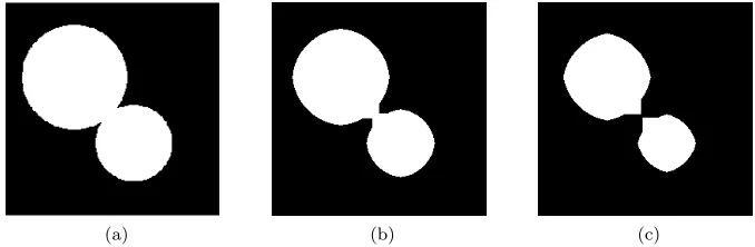
An example of the branchpoints method being applied to an image can be found in Figure 3.3. Note in this image the pointy artefacts present where a bridge between two blots has been broken up.

[image:13.612.144.483.145.256.2]

(a) (b) (c)

(14)

4. The RIMS processing method

Note: this section was written in paper format as during this thesis as we are planning to send a modified version of this chapter to the Experiments in Fluids journal. This is why some information may be repeated in this section.

4.1 Abstract

We present a method for the analysis of Refractive Index Matched Scanning (RIMS) data. RIMS is a method for the analysis of granular flow that requires a fluorescent liquid that is index matched to the particles in the system. This results in a transparent solution of particles. The fluorescent liquid is illuminated using a sheet of laser light, this means that slices of the configuration of particles in the drum can be recorded using a digital camera. By moving the sheet of laser light slightly between slices a full scan of a configuration can be made.

The RIMS method was applied to a drum that was filled with spherical particles. A tool was developed that can accurately reconstruct the configuration of particles in the drum from a set of slices. Some issues were found with the image quality of the experimental datasets. These issues could be alleviated by improving the laser illumination used in the experimental setup. The tool can be used to analyse progression of segregation in rotating drums.

4.2 Introduction

Segregation in granular materials can be analysed using a number of different techniques. Examples of such techniques are X-ray tomography [3], Magnetic Resonance Imaging (MRI) [20], optical tracking [2] and Positron Emission Particle Tracking (PEPT) [4]. The machines required for these techniques tend to be prohibitively expensive (in the order of hundreds of thousands of US dollars [26]) and most techniques are unable to capture behaviour of all particles at the same time.

Refractive Index Matched Scanning (RIMS) [5] is a relatively new technique that uses a liquid that is index matched to the material of the transparent granular particles that are being studied. This means that a vessel filled with this material and a matched liquid is transparent to the naked eye. Adding fluorescent dye to the liquid and illuminating cross sections of the vessel with a sheet of laser light makes it possible to locate cross sections of spheres due to the fact that locations where no fluorescent liquid is present stay dark, while the liquid emits light.

RIMS data can be analysed using several different methods, such as voxel-based reconstruction [27] or 2D methods [28]. For the analysis of segregation using RIMS we were interested in the locations of spheres in a glass drum. This is why a 3D reconstruction algorithm was put together. We have developed a way to process images produced using the RIMS technique and we are able to reconstruct more than 95% of the particles in the drum. In this article we will discuss the reconstruction process from start to finish.

4.3 Method

(15)

CHAPTER 4. THE RIMS PROCESSING METHOD

mixture of benzyl alcohol and ethanol. A fluorescent dye was added to the liquid.

As mentioned, the images produced using the RIMS method are cross sections of the vessel under investigation, with dark circles where the laser sheet cut through glass spheres. The drum was held by a rotating device. The slices of the drum were imaged from the front side of this drum. Images produced using this method look like Figure 4.1. Because of slight refractive index mismatches the images get blurrier as the imaged slice moves further away from the drum side from which the images are recorded, this makes the image processing step increasingly difficult.

[image:15.612.93.517.180.324.2]

(a) The first image of a dataset (b) The 100-th image of a dataset

Figure 4.1: Sample images of a RIMS dataset

The drum reconstrustion procedure was split up into two parts. In the first part the images are processed and the locations of circles are determined and stored in a text file. The second script reads this text file and reconstructs the drum using the circle locations identified using the first script.

4.3.1 Part 1: Image Processing

The first component performs a series of operations on each image in a dataset. The images are read in and a region of interest is applied to the image such that the region outside the drum is completely ignored. Then the image is analysed using a local version of Otsu’s method [32] in order to determine good threshold values for sections of the image and these threshold values are applied. Small objects in the image are removed using a set of consecutive binary opening and closing operations. After this, the image is eroded using the branchpoints procedure discussed in Section 3.5.3. Due to the order of these procedures the area originally outside the region of interest is now set to ‘true’, this region, and all elements attached to this region are eliminated by setting all elements that are in direct contact with the edges of the image to ‘false’. Some additional erosion is performed so elements that are too small are removed and now the centroids and radii of the remaining elements in the images can be determined. Multiple binary erosion operations were performed on these elements and this is compensated for by adding a constant to each recorded element radius before writing the coordinates and radii to an output file. The value of the compensation constant is equal to the number of erosion operations performed.

4.3.2 Part 2: Data Processing

(16)

After this a recursive sphere fitting algorithm identifies possible sphere fits for each of the circle groups using geometric fits [33] of variants of the circle group in multiple configurations. These configurations are then checked for overlaps with other circle groups and the configuration with conflicts are iteratively removed from the list of possible configurations until eventually a final acceptable configuration of spheres is found.

A more detailed description of Part 2 of the code can be found in Chapter 5.

4.4 Results

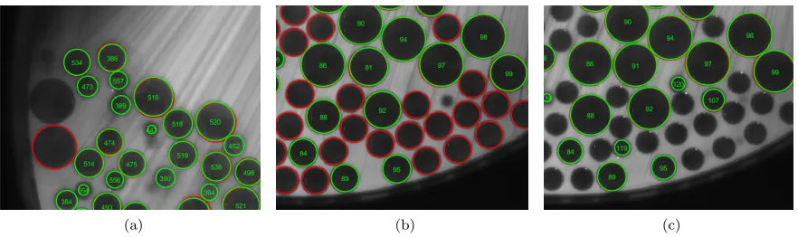
Examples of a reconstructed bidisperse and tridisperse drums can be seen in Figure 4.2. From visual inspection of the post-reconstruction control images it looks like the script correctly identifies about 95% of the particles in the drum. Some examples of unidentified spheres can be seen in Figure 4.3.

[image:16.612.97.525.265.416.2]

(a) A reconstructed bidisperse drum. (b) A reconstructed tridisperse drum

Figure 4.2: Examples of drum reconstructions.

(a) (b) (c)

[image:16.612.85.526.482.613.2]

(17)

4.5 Discussion

This analysis method for RIMS data is able to reconstruct a configuration of particles in a drum to a reasonable degree of accuracy, but there are some issues with identification of certain particles.

In the available datasets the upper edge of the bed tended to be poorly lit, which caused dark spots in those regions. An example of this lighting issue can be seen in Figure 4.3.a. A possible solution for this issue could be improving the illumination setup. This improvement could be achieved using either an additional laser sheet or by moving the laser and lens further away from the drum.

Another problem lies in the identification and fitting of small particles in the first and last slices of a dataset, which can be observed in Figure 4.3.b and Figure 4.3.c. The issue is partially caused by the fact that small particles have a diameter that is relatively small (6mm) compared to the distance between slices (1mm), this means that in Figure 4.3.c the particle slices are so small that they are ignored by the circle identification part fo the image processing script. Another part of the problem is that the first slice has to be recorded some distance away from the drum side. This distance is needed due to the way the side of the drum is glued to the cylindrical part of the drum. If the first slice is taken too close to the side of the drum then the glue causes light scattering, which creates dark and blurry spots in the image. These two issues combined lead to only one slice of these circles being found, while at least two slices of a particle are required in order to fit a sphere. A possible solution could be to either reduce the distance between slices (for example halving it to 0.5mm), but that would increase the size of datasets and also increase the time required for recording a dataset.

4.6 Recommendations

Now that drums can be reconstructed from RIMS slices and positional data can be extracted for (almost) all particles in the drum, this technique can be applied for segregation research. If slices are generated after rotating the drum a small amount, then segregation speed could be determined by computing the segregation index after each partial rotation.

(18)

5. Detailed code overview

5.1 Main code: analysis puzzle new

First a datafile is loaded in, this mat file contains a collection of circles found during image processing which has to be performed before running the main script. The images are grouped based on the image in which they were found and the circles are defined by their x and y coordinate on the image, along with their circle radius.

Pre processing

Due to the sometimes unclear nature of the images made using the RIMS technique, the image pro-cessing step sometimes finds circles in places where circles are not really present. These bad circles tend to have large overlaps with other circles, and these bad circles tend to upset sphere fitting further on in the script. So to make life a bit easier for the reconstruction part of the script, the collection of images is put under some scrutiny. Circles that have large overlaps with other circles are removed, as well as circles that are larger than the largest radius that is expected in the dataset. This step removes both the ‘bad’ circles and some ‘good’ circles, but due to the fact that there are usually plenty of slices available for each particle the accuracy of the reconstruction should not be affected much.

Circle grouping and loner removal

After the initial sanity check of the supplied dataset, grouping of the circles can start. In the initial circle grouping step circles in subsequent images are grouped if they have similar centroids. Following the initial circle grouping step is the group knitting step. In this step groups look for groups with similar centroids regardless of the distance between them. Then for all candidates the distance between the groups is calculated and if the groups are sufficiently close to each other they are linked up. Knitting of two groups is not allowed if the gap between the last circle of the first group and the first circle of the second group is greater than the radius of the first circle of the second group. This requirement is imposed in order to avoid producing large groups with multiple spheres in them, as groups like that affect the run time of the reconstruction.

After grouping and knitting, the script looks for groups with only one circle in them, called ‘loners’. These loner groups are removed from the dataset, because at least two circles are required in order to define a sphere.

Group-sphere fitting (fit alternative generation)

(19)

CHAPTER 5. DETAILED CODE OVERVIEW

For the next part of this explanation it is necessary to have a clear understanding of what is meant with ‘alternative’. An alternative is a possible single sphere fit or a configuration of multiple sphere fits that is within the acceptable error range, given the collection of data points in a set of circles grouped by the circle grouping process.

Elimination of alternatives

Now all sphere fits for all alternatives are written to a single matrix. This matrix is then used by

getcircleoverlaps()(see: Appendix D) to compute overlaps between alternatives, ignoring overlaps between spheres in the same group. Now a matrix of alternatives that have large overlaps is made, this matrix is used to decide which alternatives to discard and which ones to keep.

A boolean array of alternatives is produced in order to keep track of eliminated alternatives. Now a loop is started using which the program iteratively looks for a solution usingfindeliminators()

(see: Appendix E) anddeletefrompuzzle()(See: Appendix F) each time to try to solve the conflicts. During every iteration of the loop there are three possible outcomes:

If we have reduced the number of options (available alternatives)

Andwe have no leftover incompatibilities

1 →we are done and we canbreakthe while loop

Andwe still have leftover incompatibilites

2 →we need another iteration of the while loop to try to further reduce our options

Else if we were not able to reduce our number of available alternatives

3→then there is no point in continuing this approach and we breakthe while loop

If this procedure of eliminating possible group-sphere alternatives ends up deciding that all alterna-tives in a given circle group are unsuitable, the functionsmallestvalidoverlap()(see: Appendix G) is used to look for the least problematic option.

Now we are only left with groups with either 1 or multiple alternatives. The remaining option of groups that have only a single remaining alternative are recorded in the solution matrix of the script. All groups that still have multiple possibly valid alternatives available are stored as non-unique groups.

Determining the final configuration

These non-unique groups are processed in order to determine which of the available solutions is the most appropriate. A list of all spheres present in the alternatives is made usingcompatiblealts()

(see: Appendix H). If a sphere is present in every alternative for a given group, the sphere is accepted into the solution matrix as a unique sphere. If this still leaves the problem with non-unique spheres, then the alternative that has the lowest total fitting error is accepted. Finally all accepted spheres are checked against each other and if the overlap between the accepted spheres is within an allowable range, the spheres are stored in the final configuration.

(20)

CHAPTER 5. DETAILED CODE OVERVIEW

5.2 Function flowchart

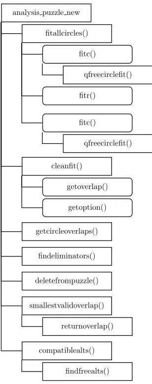
The structure of the code and its function files can be found in Figure 5.1. Sharp corners indicate standalone or parent-functions, while rounded corners indicate child-functions. The lines between boxes indicate function calls and data streams.

analysis puzzle new

fitallcircles()

fitc()

qfreecirclefit()

fitr()

fitc()

qfreecirclefit()

cleanfit()

getoverlap()

getoption()

getcircleoverlaps()

findeliminators()

deletefrompuzzle()

smallestvalidoverlap()

returnoverlap()

compatiblealts()

[image:20.612.228.382.154.541.2]

findfreealts()

(21)

6. RIMS results, progression of segregation

Note: this section was written in paper format as during this thesis as we are planning to send a modified version of this chapter to the Granular Matter journal. This is why some information may be repeated in this section.

6.1 Abstract

Segregation in a system of 6 and 9 mm particles in a slowly rotating drum with a diameter of 170 mm were analysed using the Refractive Index Matched Scanning. It was found that radial segregation took place very quickly and an intersection was found between the initial phase of fast segregation and a stable plateau at 0.64 drum rotations. This coincides with a single rotation of the particle bed.

Axial segregation was not observed within the timescale that was analysed during this project, but periodic oscillations of the segregation index were found. The cause of these oscillations is currently unclear, more data is required before solid conclusions can be drawn.

6.2 Introduction

Segregation within granular systems is something many different industries encounter. Although sev-eral efforts have been made to understand the principles behind segregation and sevsev-eral competing theories have been devised, the exact mechanisms behind segregation are still poorly understood [34]. Rotating drums are simple experimental setups using which segregation can be analysed. Other com-monly used systems are chutes [18] and vibrated systems [35].

In 1995 Cantelaube and Bideau [34] performed segregation experiments using a 2d system comprised of disks in a rotating drum. The particles in the drum were filmed. The images were then analysed using an image processing program and the progression of segregation could be determined. In the experiments 6 and 10 mm disks were used, which gives a size ratio of 1.66. The system was initially homogeneously mixed, and strong segregation was observed after only a few rotations.

In 2008 Arntz et al. [13] performed simulations of quasi-2D (narrow) drums with particles with a size ratio of 1.5. As opposed to Cantelaube and Bideau, the system was initially fully segregated: the left half of the drum was filled with small particles and the right half was filled with large particles. The progression of segregation was analysed using an entropy based segregation index. It was found that for the system under investigation at several different rotation rates, most of the rearrangement occurred in the first 10 rotations.

The goal of this research was to use Refractive Index Matched Scanning (RIMS) to determine the segregation speed of an initially-mixed drum filled with 6 and 9 mm particles.

6.3 Method

(22)

CHAPTER 6. RIMS RESULTS, PROGRESSION OF SEGREGATION

6.3.1 Experimental setup

The setup that was used was a glass rotating drum with a diameter of 170 mm and a depth of 160 mm filled with around 600 9 mm and 2100 6 mm glass spheres. The liquid used to index-match the glass drum and particles was a 69:31 mixture of benzyl alcohol and ethanol. A fluorescent dye was added to the liquid.

The setup was illuminated using a sheet of laser light. Pictures were taken from the side of the drum, generating pictures with dark spots where the laser sheet intersected glass spheres and light spots in places where fluid was present. Pictures of slices are taken with a digital camera, after each image the sheet of laser light is moved 1 mm in the axial direction of the drum.

Due to slight mismatch of the refractive index of the fluorescent light and the glass particles, the images get blurrier as the laser light moves deeper into the drum. The difference in blurriness is clearly visible in Figure 6.1.

Between scans, the drum was rotated slowly until the desired rotation was reached. Between each set of scans, the drum was rotated quite quickly in a regime where good mixing behaviour was observed (the cascading C regime as described by Arntz et al. [13]).

The datasets were analysed using the processing algorithm discussed in Chapter 4.

[image:22.612.123.515.294.433.2]

(a) The first image of a dataset (b) The 100-th image of a dataset

Figure 6.1: Sample images of a RIMS dataset

6.3.2 Mixing state characterisation

After reconstruction of the particle positions in the drum, the progession of segregation could be analysed. In order to characterise the state of the system at different points in time, the segregation index as described by Arntz[36] was used. This is a segregation indicator based on Boltzmann’s expression (Equation (6.1)). In this equationxa(k) andxb(k) are the number fractions of species a and b in cellkands(k) is the local entropy in cellk. A cell is a section of the drum. The cell size can be chosen freely, but a cell should be smaller than the expected size of segregation features. During post processing multiple cell sizes were tested and compared against each other.

s(k) =xa(k) lnxa(k) +xb(k) lnxb(k) (6.1)

Summing these local entropies and multiplying by the number of particles in each cell (denoted as

n(k, t)) gives the total entropy at any timestep S(t) (Equation (6.2)). WhereN is the total number of particles in the system.

S(t) = 1

N X

k

s(k, t)n(k, t) (6.2)

(23)

φ(t) = S(t)−Sseg

Smix−Sseg

(6.3)

Arntz [36] defined systems to be mixed ifφ >0.9 and segregated ifφ <0.65. Though this definition is only valid if the cell size,Smixand Sseg are chosen correctly.

By determining the location of the spheres after multiple partial rotations, the segregation speed can be determined. By defining cells in the plane of the side of the drum radial segregation speed can be determined. By choosing to define cells in the plane of the front or top of the drum progression of axial segregation can be determined.

As we are aware that the reconstruction algorithm sometimes fails to include all spheres in the final configuration, sensitivity checks have to be performed in order to determine how sensitive the segregation index trend is to missed datapoints.

6.4 Results and Discussion

In this section the results and discussion of the experiments are presented. First the segregation speed is analysed in the radial and axial directions. Another result that will be shown is the effect of choosing several different bin widths on the segregation index. Finally also measurements of axial segregation are presented.

6.4.1 Radial segregation

[image:23.612.133.477.413.646.2]

Of main interest was the radial segregation speed of the mixture of 6 and 9 mm particles. Figure 6.2 shows the progression of segregation when the values forSseg =−0.05 andSmix=−0.52 are used in Equation (6.3) with a cell size of 25mm.

Figure 6.2: Progression of radial segregation in a slowly rotating drum. For all datasets Segregation Index parameters are set toSseg =−0.05 andSmix=−0.52 and a bin width and height of 25 mm.

(24)

of the drum and the segregated state after one drum rotation is shown in Figure 6.3. In the initial state the drum appears well mixed. During inspection of the inside of the reconstruction it appears as though particles are distributed randomly in the drum. There is a slight bias for large particles the the bottom part of the free surface. This bias is likely caused by the way the drum is stopped at the end of the mixing cycle.

The configuration of the particles in the drum after one rotation was analysed similarly. A core of small particles in centre of the particle bed is now clearly present. The core is surrounded by a shell of mostly large particles. Such configurations are typical for slowly rotating bidisperse mixtures [13].

[image:24.612.111.517.197.330.2]

(a) Initial drum configuration. (b) Drum configuration after a full rotation.

Figure 6.3: Side views of reconstructed drums.

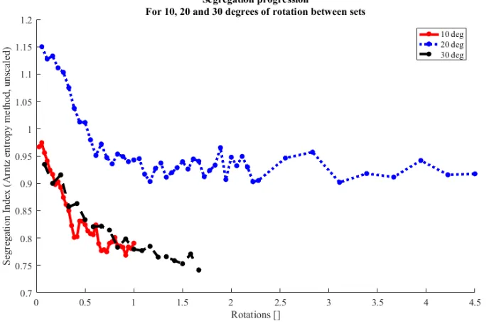
The difference in starting segregation index could be compensating by selecting different values for the reference segregation stateSmix(shown in Figure 6.4). The initial value of the segregation index was shifted to 1 by settingSmix to -0.509 for the 10 degree set, -0.59 for the 20 degree set and -0.49 for the 30 degree set. The value for the 20 degree set is quite far removed from the 10 and 30 degree set. This can be explained by the fact that in the 20 degree set the ratio between the number of large and small particles is 0.41 instead of the ratio of 0.29 that was used for the 10 and 30 degree sets. This difference in number ratio results in a reference situation.

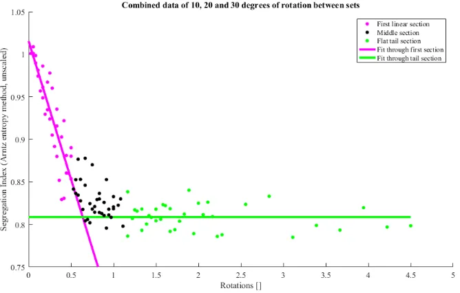
Figure 6.4: Progression of segregation in a slowly rotating drum. For all datasets segregation index parameterSseg=−0.05,Smixwas set to the values listed in the legend in order to normalise the data.

[image:24.612.138.473.478.674.2]

(25)

[image:25.612.138.472.166.379.2]

initial phase of rapid segregation was fitted with a linear fit. The plateau region was fitted with a line at the average value of the datapoints in the equilibrium region. The two fits intersect at approximately 0.64 rotations. This corresponds almost perfectly with the ratio of the circumference of the particle bed and the circumference of the drum. This possible relation could be tested by performing new experiments at different fill levels.

Figure 6.5: Progression of segregation in a slowly rotating drum with 6 and 9 mm particles. Datasets were normalised as in Figure 6.4. Linear fits were made through the initial linear section (indicated in magenta) and through the flat tail part of the data (indicated in green).

Effects of bin width

The bin size in the segregation index calculation is a factor that can influence the results. This is why a sensitivity analysis was performed for this parameter. The same datasets were analysed using different bin widths and presented in Figure 6.6. It appears as though slightly increasing the bin width slightly changes peaks in the data. This could be due to the fact that particles near the edges a bin suddenly belong to a different cell. This changes the particle ratios within the cells computed using Equation (6.1).

(26)

[image:26.612.198.402.85.225.2]

Figure 6.6: Sensitivity check of the influence of bin with during calculation of the segregation index.

6.4.2 Axial segregation

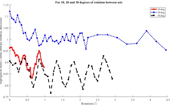
The progression of axial segregation was the subject of another analysis, shown in Figure 6.7. None of the datasets showed significant signs of axial segregation. For the 10 and 30 degree datasets, however, a strange trend was observed. These sets showed oscillations that were in phase with each other.

This could be caused by a cluster of particles that moves through the drum periodically. The period of the oscillation is the same as the ratio between a bed rotation and a drum rotation (0.64). Another possible cause could be a periodic reduction of the image quality due to contaminations on the wall of the drum. At this point the exact cause of the oscillation is still unclear.

Figure 6.7: Progression of axial segregation index in a slowly rotating drum. For all datasets Segrega-tion Index parameters are set toSseg =−0.05 and Smix=−0.52. The horizontal bin width was set to 25 mm, while the axial bin width was 10 mm.

6.5 Conclusion and outlook

[image:26.612.158.453.387.569.2]

(27)

(28)

Bibliography

[1] Matthias E M¨obius, Benjamin E Lauderdale, Sidney R Nagel, and Heinrich M Jaeger. Brazil-nut effect: Size separation of granular particles. Nature, 414(6861):270, 2001.

[2] Sudeshna Roy, Bert J Scheper, Harmen Polman, Anthony R Thornton, Deepak R Tunuguntla, Stefan Luding, and Thomas Weinhart. Surface flow profiles for dry and wet granular materials by particle tracking velocimetry; the effect of wall roughness. arXiv preprint arXiv:1901.01472, 2019.

[3] Athanasios G Athanassiadis, Patrick J La Rivi`ere, Emil Sidky, Charles Pelizzari, Xiaochuan Pan, and Heinrich M Jaeger. X-ray tomography system to investigate granular materials during mechanical loading. Review of Scientific Instruments, 85(8):083708, 2014.

[4] DJ Parker, AE Dijkstra, TW Martin, and JPK Seville. Positron emission particle tracking studies of spherical particle motion in rotating drums. Chemical Engineering Science, 52(13):2011–2022, 1997.

[5] S´ebastien Wiederseiner, Nicolas Andreini, Ga¨el Epely-Chauvin, and Christophe Ancey. Refractive-index and density matching in concentrated particle suspensions: a review. Experiments in fluids, 50(5):1183–1206, 2011.

[6] Heinrich M Jaeger, Sidney R Nagel, and Robert P Behringer. Granular solids, liquids, and gases.

Reviews of modern physics, 68(4):1259, 1996.

[7] M Bose, UU Kumar, PR Nott, and V Kumaran. Brazil nut effect and excluded volume attraction in vibrofluidized granular mixtures. Physical Review E, 72(2):021305, 2005.

[8] Patrick Richard, Mario Nicodemi, Renaud Delannay, Philippe Ribiere, and Daniel Bideau. Slow relaxation and compaction of granular systems. Nature materials, 4(2):121, 2005.

[9] Janet Cho, Yunfeng Zhu, Karol Lewkowicz, SungHee Lee, Theodore Bergman, and Bodhisattwa Chaudhuri. Solving granular segregation problems using a biaxial rotary mixer. Chemical Engi-neering and Processing: Process Intensification, 57:42–50, 2012.

[10] John Mark Nicholas Timm Gray. Particle segregation in dense granular flows. Annual Review of Fluid Mechanics, 50:407–433, 2018.

[11] Andrew M Scott and John Bridgwater. Interparticle percolation: a fundamental solids mixing mechanism. Industrial & Engineering Chemistry Fundamentals, 14(1):22–27, 1975.

[12] A Alexander, FJ Muzzio, and T Shinbrot. Effects of scale and inertia on granular banding segregation. Granular Matter, 5(4):171–175, 2004.

[13] MMHD Arntz, Wouter K den Otter, Willem J Briels, PJT Bussmann, HH Beeftink, and RM Boom. Granular mixing and segregation in a horizontal rotating drum: a simulation study on the impact of rotational speed and fill level. AIChE journal, 54(12):3133–3146, 2008.

(29)

BIBLIOGRAPHY

[15] R´emi Jullien, Paul Meakin, and Andr´e Pavlovitch. Three-dimensional model for particle-size segregation by shaking. Physical Review Letters, 69(4):640, 1992.

[16] Troy Shinbrot and Fernando J Muzzio. Reverse buoyancy in shaken granular beds. Physical Review Letters, 81(20):4365, 1998.

[17] Deepak R Tunuguntla, Thomas Weinhart, and Anthony R Thornton. Comparing and contrasting size-based particle segregation models. Computational Particle Mechanics, 4(4):387–405, 2017.

[18] SB Savage and CKK Lun. Particle size segregation in inclined chute flow of dry cohesionless granular solids. Journal of Fluid Mechanics, 189:311–335, 1988.

[19] DV Khakhar, Ashish V Orpe, and SK Hajra. Segregation of granular materials in rotating cylinders. Physica A: Statistical Mechanics and its Applications, 318(1-2):129–136, 2003.

[20] Masami Nakagawa, SA Altobelli, A Caprihan, E Fukushima, and E-K Jeong. Non-invasive mea-surements of granular flows by magnetic resonance imaging. Experiments in fluids, 16(1):54–60, 1993.

[21] Kimberly M Hill, Arvind Caprihan, and James Kakalios. Bulk segregation in rotated granular material measured by magnetic resonance imaging. Physical Review Letters, 78(1):50, 1997.

[22] Ralf Stannarius. Magnetic resonance imaging of granular materials. Review of Scientific Instru-ments, 88(5):051806, 2017.

[23] DJ Parker, RN Forster, P Fowles, and PS Takhar. Positron emission particle tracking using the new birmingham positron camera. Nuclear Instruments and Methods in Physics Research Section A: Accelerators, Spectrometers, Detectors and Associated Equipment, 477(1-3):540–545, 2002.

[24] John C Crocker and Eric R Weeks. Particle tracking using idl.Retreived from http://www. physics. emory. edu/faculty/weeks//idl, 2011.

[25] Linbing Wang, Jin-Young Park, and Yanrong Fu. Representation of real particles for dem simu-lation using x-ray tomography. Construction and Building Materials, 21(2):338–346, 2007.

[26] Joshua A Dijksman, Frank Rietz, Kinga A L˝orincz, Martin van Hecke, and Wolfgang Losert. Invited article: Refractive index matched scanning of dense granular materials.Review of Scientific Instruments, 83(1):011301, 2012.

[27] Joshua A Dijksman, Nicolas Brodu, and Robert P Behringer. Refractive index matched scanning and detection of soft particles. Review of Scientific Instruments, 88(5):051807, 2017.

[28] Kasper van der Vaart, Parmesh Gajjar, Ga¨el Epely-Chauvin, Nicolas Andreini, JMNT Gray, and Christophe Ancey. Underlying asymmetry within particle size segregation.Physical review letters, 114(23):238001, 2015.

[29] Kasper van der Vaart, AR Thornton, CG Johnson, T Weinhart, L Jing, P Gajjar, JMNT Gray, and C Ancey. Breaking size-segregation waves and mobility feedback in dense granular avalanches.

Granular matter, 20(3):46, 2018.

[30] John C Russ. The image processing handbook. CRC press, 2016.

[31] John C Crocker and David G Grier. Methods of digital video microscopy for colloidal studies.

Journal of colloid and interface science, 179(1):298–310, 1996.

[32] Nobuyuki Otsu. A threshold selection method from gray-level histograms. IEEE transactions on systems, man, and cybernetics, 9(1):62–66, 1979.

(30)

BIBLIOGRAPHY

[34] F Cantelaube and D Bideau. Radial segregation in a 2d drum: an experimental analysis. EPL (Europhysics Letters), 30(3):133, 1995.

[35] James B Knight, Heinrich M Jaeger, and Sidney R Nagel. Vibration-induced size separation in granular media: The convection connection. Physical review letters, 70(24):3728, 1993.

(31)

(32)

A. Function: fitallcircles()

A.1 fitallcircles()

Outputs

Par, [x - 0 - r] Parameters of the circle fits

err, a list of allowed fit errors per datapoint divided by the circle radius

cutoffs, in the case that a circle group contains more than one sphere, this list indicates where one sphere ends and another starts

overlap, in the case that a circle group contains more than one sphere, this lists the overlaps between the spheres

Inputs

XY, [x - r] x-coordinates and radii of circles in a circle group

radii, a list of radii that are expected in the system

varargin

‘verbose’, makes the code output messages to the command line

‘free’, allows free geometric fitting in the fitc() subfunction (so no information about ex-pected circle radius is exex-pected)

‘all’, makes the function return all fits, without checking whether the errors of the fits are within acceptable bounds

‘bitfree’, expects an additional input: the allowed deviation of the fit radius from the radii in radii. If the function is in bitfree mode, the circle fitting is a little bit free, the radius of the circle fits are tested against the supplied radii, but some deviation is allowed

fitallcircles() code explanation

First the input inXYis sorted and the output variables are initalised as empty cell arrays. After this a loop is entered wherein an attempt is made to fit circles to the supplied datasets. The actual fitting is done by subfunctionfitr(), which stands for ‘fit recursively’. fitr()returns the same outputs as

(33)

APPENDIX A. FUNCTION: FITALLCIRCLES()

A.2 Subfunction: fitr() of fitallcircles()

Outputs

The outputs offitr() are the same as the outputs of its parent function fitallcircles()but the parent function inspects the outputs and rejects unsuitable fits.

cutoffs, in the case that a circle group contains more than one sphere, this list indicates where one sphere ends and another starts

overlap, in the case that a circle group contains more than one sphere, this lists the overlaps between the spheres

Inputs

count, the number of recursive loops already performed, in other words: the recursive depth of the current solution

maxcount, the maximum number of recursive loops that is allowed in order to obtain a fit

fitr() code explanation

This function is a recursive function, which means that it is a function that can call another instance of itself. This is done in an effort to reduce the problem until a state is reached in which it becomes simple to solve the reduced problem. This recursive function essentially has two possible outcomes: in the first case the problem at hand is simple and the function can solve the problem, this is called the

base case. The second possible outcome is that the problem is too complicated to solve immediately, in this case the problem is reduced further and another instance of the function is called, this is known as therecursive case.

In the base case all entries inXY are fed to the subfunction called fitc() and fitc()returns a circle fit for the given datapoints and also returns the average fitting error per datapoint divided by the circle radius.

If the problem is not simple enough for the base case, therecursive caseis called. Here a for-loop is used to send part of the circle group to the function calledfitc()(see: Appendix A.3) and the other part is fed into another instance offitr() (so the function calls a new instance of itself, hence the ‘recursive’ in the function name). These recursive functions compute partial solutions for the fitting problem and all these partial solutions are added to the solution of the main problem if their fits have sufficiently low fitting errors.

(34)

A.3 Subfunction: fitc() of fitr() (of fitallcircles())

Outputs

Inputs

fitc() code explanation

This function tries to fit a single circle to the [x - r] data in XY. There are three possible ways this function can be performed:

If the supplied dataset inXYonly contains a single circle

→no sphere can be fitted to the dataset and the data is returned as a loner in the shape [x - r - 0]

Else if XYcontains exactly 2 circles

→a sphere can be fitted geometrically. This is done using the following method:

The horizontal distance Dx between the datapoints is computed, as well as d1 (using Equa-tion (A.1)), R (using Equation (A.2)) and d2 (using Equation (A.3)). The meaning of these parameters is illustrated in Figure A.1. Now usingd1andd2the centrepoint of the fitted circle can be determined as follows:

If abs(Dx-d1-d2) is very small

→The centre of the circle is between the two given datapoints

Elseif d2>d1

→The centre is to the left of both datapoints

Else(d1>d2)

→The centre is to the right of both datapoints

If there are more than 2 datapoints or if geometric fitting returns an unnaceptable fit

→qfreecirclefit()is called in order to fit the dataset

d1 = abs(R 2

1−R22−Dx2)

2Dx (A.1)

R=

q R2

1+d21 (A.2)

d2 =

q

R2₋_R2

(35)

[image:35.612.198.413.92.201.2]

(36)

B. Function: qfreecirclefit()

The function is called byfitc() as: [Par,err]=qfreecirclefit(xy,‘bitfree’,radii,dr)Where radii contains the given particle radii in pixels and dr contains the maximum allowable fit error in pixels (this value is set to 5.5 pixels).

Outputs

xyr, [x - y - r] (in the output of this function y is always equal to 0)

err, the average error per datapoint divided over radius

Inputs

data, [x - r]

varargin

’rmax’, for setting max radius

’rrange’, for setting a minimum and maximum radius

’bitfree’, takes both a set of radii (radii) and a maximum allowable fitting error in pixels (dr). First a check is performed to see which of the radii best matches the input and then the search area for the actual fit becomes the found radius plus and minus the allowable fit error

qfreecirclefit() code explanation

The code starts by storing the first and last radius of the dataset inxyin y1and yend, the same is done with the first and last x-coordinates inx1andxend. After this the search space for the circle fit has to be determined. The search space is set to the space betweenxminandxmax.

If the input dataset contains more than 2 circles and the maximum radius in the set does not belong to the the first or the last circle (Case 1 in Figure B.1) then:

→ xminis the x-coordinate of the first circle

→ xmaxis the x-coordinate of the last circle

Else if the last radius>the first radius (Case 2 in Figure B.1).

→ xminis the x-coordinate of the first circle

→ xmaxisxmin plus the largest possible radius

Elsethe last radius<the first radius (Case 3 in Figure B.1).

→ xmaxis the x-coordinate of the last circle

(37)

[image:37.612.150.464.84.166.2]

APPENDIX B. FUNCTION: QFREECIRCLEFIT()

Figure B.1: The three possible cases for a given dataset with of datapoints (illustrated as blue dots).

After this a radius search space is made in r the search space is initially set for all given radii in xlength (= 5) steps between radii(i)-dr and radii(i)+dr, where i indicates the i-th possible radius.

Another search space is made for the x-location of the sphere. This is done in di*xlength(=10) steps betweenxminandxmax.

The search areas are now iteratively narrowed down for every combination of the entries in the search spaces for the x location and the radius. If the current x location is called the trial point, then the distance between the trial point and each datapoint is stored as the implied radiusri. Then the differences between all entries in the radius search space can be computed using Equation (B.1) where

F is the sum of the squared errors, ri is the current set of implied radii and r(j) is the currently tested radius. Figure B.2 shows how the implied radii are computed for a given trial point.

F =sum((ri−r(j))2) (B.1)

Figure B.2: The implied radius method. The blue dot is an example of a trial point, the red dots are datapoints and the dashed straight lines show the implied radii. In this example the trial point is quite far away from the actual centre of the circle.

During the calculation ofF,if the currentFis the smallest one so far, the current value is stored as the new minimum value ofFand the current trial point and trial radius are also stored. If the current value ofFis sufficiently small the search is stopped and the found midpoint of the circle and its radius are given as output.

If a sufficiently good fit is not yet found, the search space is narrowed down based on the previously found minimum fit error:

→ For the x-coordinate, the search area is reduced to the locations between the neighbour of the previously found minimum error squared (see Figure B.3).

→ For the radius, in the first iteration of the search the most appropriate radius is selected from the list of available radii and the search space is set to radius-dr andradius+dr. In subsequent iterations the search space is set to between the neighbours of the local minimum error squared (see Figure B.3).

[image:37.612.198.409.351.487.2]

(38)

APPENDIX B. FUNCTION: QFREECIRCLEFIT()

[image:38.612.203.405.136.253.2]

that the fitting error is within the allowed error margin) is found and the good fit is returned as the function output along with the fit error divided by the number of datapoints and the found radius.

(39)

C. Function: cleanfit()

C.1 cleanfit()

Outputs

newPar, [x - 0 - r] Parameters of the new circle fits, at this point, the second column in the matrix is still 0 because this stage of the script is still dealing with 2D fitting

overlap, overlaps between circles divided by the radius of the biggest circle involved in the overlap

Inputs

Par, [x - 0 - r] Parameters of circle fits, at this point, the second column in the matrix is still 0 because this stage of the script is still dealing with 2D fitting

varargin

‘verbose’, makes the code output more messages to the command line

‘bitfree’, expects an additional input: the allowed deviation of the fit radius from the radii in radii. If the function is in bitfree mode, the circle fitting is a little bit free, the radius of the circle fits are tested against the supplied radii, but some deviation is allowed

cleanfit() code explanation

The code starts out by finding loner indices in the provided set of circles inPar. Loners in this case are circles that do not belong to a fitted sphere. These so called ‘loners’ are found using the fact that the program up to now has stored fitted circles as [x 0 r], while it has stored loners in the form [x -r - 0].

(40)

[image:40.612.196.418.91.233.2]

APPENDIX C. FUNCTION: CLEANFIT()

Figure C.1: Illustration of the circles identified as possible fits for a given loner. In this image the blue dot indicates the x-coordinate of the loner, while the distance between the blue and red dot indicates the loner radius. In this example two available radii were available to this loner. Circles from the smaller available radius are shown in dark grey, while the circles belonging to the larger radius are shown in a lighter grey.

These possible loner fits are checked for overlap with other spheres in the dataset inParand if the overlap with other non-loner circles in the dataset is too large then the loner option is removed from the list of options. If none of the options is valid then the outputsnewParand overlapare returned empty. If, however, there are valid options then the invalid options are removed and we check if the removal of these options also reduces the options for the previous sphere. If options for the previous sphere are not reduced, then we check if options for the next sphere can be reduced.

(41)

APPENDIX C. FUNCTION: CLEANFIT()

C.2 Subfunction: getoption() of cleanfit()

Outputs

op, [option 1 - option 2 - ... - option n] contains the requested option number configuration

Inputs

nop, [noptions,sphere1- noptions,sphere2- ... - noptions,lastsphere] contains the number of options for each sphere in theParset thatcleanfit()is currently working on.

x, the currently requested configuration of options

getoption() code explanation

This function does not perform a puzzling step per se, but it performs a mathematical operation. This is why the explanation style is a bit different from the one used for the other functions and subfunctions.

This function takes the total number of particles and the number of options available to these options and a requested configuration number and it returns an option configuration corresponding to this configuration number.

For example, if the current group of spheres has 3 available options for the last 2 of 3 spheres with the first sphere only having a single option, then inputnopwould be [1,3,3] and we would have 1∗3∗3 = 9 available options with the configuration numbers and corresponding configurations as seen in Table C.1.

Table C.1

configuration numberx configuration

1 [1,1,1]

2 [1,1,2]

3 [1,1,3]

4 [1,2,1]

5 [1,2,2]

6 [1,2,3]

7 [1,3,1]

8 [1,3,2]

(42)

D. Function: getcircleoverlaps()

Outputs

overl, [spherenumber 1 - spherenumber 2 - overlap - relative overlap] a list of overlapping spheres, along with their overlap as well as the overlap divided by the radius of the smallest of the spheres involved in the overlap

Inputs

XYR, [x - y - z- r] in 3D or [x - y - r]

varargin

‘verbose’, makes the code output more messages to the command line

getcircleoverlaps() code explanation

First a box is defined that contains all spheres present in the system. This box is then divided up into smaller cells, such that a sphere within any given cell can only be in contact with spheres that are in that same cell or any of the 26 cells that neighbour that cell.

(43)

E. Function: findeliminators()

Outputs

eliminators, [group number - alternative number] this is a list of eliminators. An eliminator is a group alternative that has conflicts with all alternatives of another group

eliminated, [group number - alternative number] this is a list of eliminated group alternatives

Inputs

bga, this variable contains a Boolean Grid Array of all groups and alternatives present in the system. Each row of the array represents a group in the puzzle and every column represents an altnumber that is still available to that group. It is possible for a group’s row to look like [1,0,0,1], this would mean that this group still has alt number one and four available and that alt number two and three have been eliminated.

inc, [groupnumber 1 - altnumber 1 - groupnumber 2 - altnumber 2] a list of groups and alternatives that are incompatible with each other. In this case incompatible means that the two groups can not both be in the final solution of the puzzle as they have a relative overlap that is too large.

findeliminators() code explanation

A list of groups with incompatibilities is made and a loop is performed over all entries in this list. For each entry in the list a smaller list with all group alternatives that are incompatible with the current group is made. Then a check is performed to see if the groups involved in the incompatibilities are

A Code for Refractive Index Matched Scanning Data Processing

A Code for Refractive Index Matched

Scanning Data Processing

Contents

1.

Summary

2.

Introduction

3.

Background

3.1

Granular materials

3.2

Granular segregation

3.2.1

Size segregation

3.3

Methods for the analysis of granular systems

3.3.1

Magnetic Resonance Imaging

3.3.2

Positron Emission Particle Tracking

3.3.3

Optical tracking

3.3.4

X-ray tomography

3.4

Previous work on RIMS

3.5

Image processing for RIMS

3.5.1

Convolution

3.5.2

Watershed

3.5.3

Applied method: branchpoints

4.

The RIMS processing method

4.1

Abstract

4.2

Introduction

4.3

Method

4.3.1

Part 1: Image Processing

4.3.2

Part 2: Data Processing

4.4

Results

4.5

Discussion

4.6

Recommendations

5.

Detailed code overview

5.1

Main code: analysis puzzle new

5.2

Function flowchart

6.

RIMS results, progression of segregation

6.1

Abstract

6.2

Introduction

6.3

Method

6.3.1

Experimental setup

6.3.2

Mixing state characterisation

6.4

Results and Discussion

6.4.1

Radial segregation

6.4.2

Axial segregation

6.5

Conclusion and outlook