Development of solid state NMR to understand materials involved in catalytic technology used in fuel cells

(1)

University of Warwick institutional repository: http://go.warwick.ac.uk/wrap

A Thesis Submitted for the Degree of PhD at the University of Warwick

http://go.warwick.ac.uk/wrap/50241

This thesis is made available online and is protected by original copyright.

Please scroll down to view the document itself.

(2)

AUTHOR:Gregory Jon Rees DEGREE:Ph.D.

TITLE:Development of Solid State NMR to Understand Materials Involved in Catalytic Technology used in Fuel Cells

DATE OF DEPOSIT: . . . .

I agree that this thesis shall be available in accordance with the regulations governing the University of Warwick theses.

I agree that the summary of this thesis may be submitted for publication. I agree that the thesis may be photocopied (single copies for study purposes only).

Theses with no restriction on photocopying will also be made available to the British Library for microfilming. The British Library may supply copies to individuals or libraries. subject to a statement from them that the copy is supplied for non-publishing purposes. All copies supplied by the British Library will carry the following statement:

“Attention is drawn to the fact that the copyright of this thesis rests with its author. This copy of the thesis has been supplied on the condition that anyone who consults it is understood to recognise that its copyright rests with its author and that no quotation from the thesis and no information derived from it may be published without the author’s written consent.”

AUTHOR’S SIGNATURE: . . . .

USER’S DECLARATION

1. I undertake not to quote or make use of any information from this thesis without making acknowledgement to the author.

2. I further undertake to allow no-one else to use this thesis while it is in my care.

DATE SIGNATURE ADDRESS

. . . .

(3)

Development of Solid State NMR to Understand

Materials Involved in Catalytic Technology used in

Fuel Cells

by

Gregory Jon Rees

Thesis

Submitted to the University of Warwick

for the degree of

Doctor of Philosophy

Department of Physics

(4)

List of Tables

4.1 Experimental Pulsed NMR Parameters used for the Various Nuclei . 81 4.2 Theoretical and experimental values for the relative intensities of the

different regions based on a total atom number five layered nanoparticle. 83 4.3 A comparison of the theoretical model against the deconvolution of

the platinum sweeps for various platinum nanoparticle sizes. . . 88 4.4 Experimentally measured 195-Pt and 119-Sn NMR interaction

pa-rameters for PtYSnX bimetallics systems. . . 91 4.5 Relaxation Times of Platinum-X Alloys and Intermetallics . . . 96

5.1 Experimentally measured and NMR-CASTEP DFT calculated 17O NMR interaction parameters for various apatite systems. . . 115

6.1 Experimentally measured and NMR-CASTEP DFT calculated 1H Isotropic shifts and 13C CSA parameters . . . 137 6.2 Experimentally measured and NMR-CASTEP DFT calculated 17O

Isotropic shifts and Quadrupolar parameters . . . 142 6.3 A comparison of the solid state NMR data achieved for the group IA

metals with their corresponding DFT-CASTEP data . . . 148 6.4 A Comparison of Techniques used to Define Hydrogen Bonding

Char-acter . . . 150

(10)

List of Figures

2.1 Euler angle rotations . . . 10

2.2 The Legendre polynomials . . . 12

2.3 Zeeman Splitting of Common Nuclei . . . 15

2.4 Chemical Shift Anisotropy . . . 20

2.5 Quadrupole Coupling Constant (CQ) and Asymmetry parameter (η) 22 2.6 Euler Angles . . . 28

2.7 Magic Angle Spinning . . . 33

3.1 Longitudinal Relaxation . . . 47

3.2 Free induction decay during static and MAS experiments . . . 48

3.3 Nutation rates in yttrium aluminium garnet . . . 52

3.4 A one pulse NMR experiment . . . 54

3.5 Spin echo . . . 55

3.6 Chemical shift ranges of some the spin-1₂ nuclei . . . 58

3.7 QCPMG pulse sequence . . . 62

3.8 Coherence pathway of a Z-Filter MQMAS . . . 65

3.9 DOuble rotation . . . 69

4.1 Field Sweep Fourier Transform of a Platinum Nanoparticle . . . 82

4.2 Comparison of Wideline NMR Techniques on a Platinum Nanoparticle 84 4.3 Comparison of Spin Echo Height Spectroscopy and Field Sweep Fourier Transform NMR on varying sizes of Platinum Nanoparticles . . . 86

4.4 Platinum 13 Clusters . . . 90

4.5 NMR and X-ray Crystallography of Platinum - Tin Intermetallics . . 92

4.6 Alloys and their corresponding Metals . . . 93

4.7 Platinum NMR and X-ray Crsytallography of Alloys . . . 95

(11)

5.2 The Density Functional Theory CASTEP determined spectra for

sample lanthanum-yttrium germanate . . . 105

5.3 The silicon MAS and oxygen MAS NMR Spectra of Rare Earth Sili-cate Oxide Ion Conductors . . . 107

5.4 The oxygen MAS NMR of Rare Earth Germanate Oxide Ion Conductors110 5.5 The Quadrupole Coupling Parameters, MQMAS and Calculated Pa-rameters for the Silicates and Germanates . . . 113

5.6 3QMAS Spectra of highly labelled Apatite Ion Conductors . . . 117

5.7 DOR Spectra of highly labelled Apatite Ion Conductors . . . 118

5.8 Proton Mobility Spectra for Determination of the Water and Hy-droxyl Environment in Apatites . . . 119

6.1 Chemical Shift Anisotropy Tensors of Carboxylic Gropus . . . 125

6.2 Crystal Structures of the Hemibenzoates . . . 131

6.3 The Packing Structures of the Hemibenzoates . . . 133

6.4 The Fast MAS Proton Solid State NMR of the Hemibenzoate Series 135 6.5 Chemical Shift Anisotropy of the Carboxy Group in the Hemiben-zoate Series . . . 139

6.6 17-Oxygen MAS NMR of the Hemibenzoate Series . . . 141

6.7 17-Oxygen DOR NMR of the Hemibenzoate Series . . . 144

6.8 The Calculated Isotropic Shift and Quadrupole Parameter for the Hemibenzoate Series . . . 146

6.9 NMR of the Group IA Metals . . . 147

(12)

Acknowledgments

Without the help, guidance and instruction of the following people none of the work

presented here in this thesis would be possible. I would like to express my gratitude

to my supervisors Dr John Hanna and Prof. Mark Smith, whose support, expertise,

knowledge and understanding added considerably towards my research experience.

Beside my supervisors, I would like to express thanks to Dr Andrew Howes for

his technical expertise and his immense patience when it came to the double rotation

experiments present in this thesis. I am indebted to my many of my colleagues who

have offered me guidance and generally useful discussions throughout my research

and thesis writing, these include Scott King, Dr Thomas Partridge, Stephen Day,

Andrew Tatton, Prof. Ray Dupree, Dr Simon Orr, Dr Lindsay Cahill, Dr Nathan

Barrow, Dr Jonathan Bradley, Prof. Steven Brown, Dr Dinu Iuga, Dr Kevin Pike

and Dr Thomas Kemp.

I am grateful for all the help supplied by my collaborators. At Johnson

Matthey the advice supplied from Dr David Thompsett, Dr Jennifer Houghton, Dr

Janet Fischer and Dr Geoffrey Spikes was appreciated greatly. Prof. John Wallis

and Dr Alberth Lari (Nottingham Trent University) gave me a massive amount of

assistance and advice when it came to the organic sections of my thesis; discussions

with them both were greatly valued. I am grateful for the high quality labeled

apatite samples and knowledge offered by Dr Peter Slater and Dr Alodia Orera

from the University of Birmingham.

I would also like to thank my parents, brother, sister and grandparents (past

and present) for the support they provided throughout my academic studies. I also

(13)

given me a huge amount of lift during rocky times.

Finally, I recognise that this research would not have been possible without

the financial backing from the Engineering and Physical Science Research Council

(EPSRC), Johnson Matthey and the University of Warwick.

(14)

Declarations

I hereby declare that this dissertation entitledDevelopment of solid state NMR to understand materials involved in catalytic technology used in fuel cells

is an original work and has not been submitted for a degree or diploma or other

qualification at any other University.

Results from other authors are referenced in the usual manner throughout

the text. All collaborative results are indicated in the text along with the nature

and extent of my individual contribution, a brief summary is given here:

In the chapter 4 all the samples were supplied and synthesised by partners

at Johnson Matthey Technology Centre, UK. Johnson Matthey’s in house analysis

facilities supplied the X-ray diffraction results.

In the chapter 5 the samples were synthesised by Dr. Alodia Orera and

Dr. Peter Slater at the University of Birmingham, the published density functional

theory calculations in reference [1] by Dr. Pooja Panchmatia were duplicated in our

laboratory to give greater accuracy and were simulated by myself.

All samples and X-ray diffraction present in chapter 6 were supplied by

col-laboraters Dr. Alberth Lari and Prof. John Wallis from Nottingham Trent

(15)

Abstract

The utility of the little used Field Sweep Fourier transform (FSFT) method is

demonstrated for recording wideline nuclear magnetic resonance (NMR) of195_Pt

res-onances for various sized platinum nanoparticles, as well as platinum-tin bimetallics

used in fuel cell catalysts, and various other related platinum (Pt3X; X = Al, Sc,

Nb, Ti, Hf and Zr) alloys. The lineshapes observed from PtSn for both 195Pt and

119_{Sn suggest that it is more ordered than other closely related intermetallics, which}

might be expected from other measurements (e.g. XRD linewidths). From these

reconstructed spectra the mean number of platinum atoms in the nanoparticle can

be accurately determined along with detailed information regarding the number of

atoms present effectively in each layer from the surface. This can be compared with

theoretical predictions of the number of platinum atoms in these various layers for

cubo-octahedral nanoparticles, thereby providing an estimate of the particle size. A

comparison of the common NMR techniques used to acquire wideline spectra from

spin I = 1₂ nuclei shows the advantages of the automated FSFT technique over

the spin echo height/integration approach that dominates the literature. A study

of small 13 atom platinum clusters, with variable particle size dispersion for which

there is no experimental characterisation in the literature, provides evidence for an

isotropic chemical shift of these platinum nanoparticles and provides a better basis

for determining the Knight shift when compared to referencing against the primary

IUPAC standard which has a different local structure.

Rare earth apatite oxide ion conductors are novel candidates for electrolytes

(16)

conductor at lower temperatures when compared to the market leader yttrium

sta-bilised zirconia (YSZ). To understand the mechanism of its conduction 17O-labelled

water was allowed to conduct through the sample and 17O solid state NMR was

employed to comment on this pathway in a series of germanium and silicon

sub-situted apatites. The linear channels running through the centre of the structure

were believed to contain vacancies and as with perovskites it was commonly believed

these allowed hopping of the oxygen to enable the apatite to conduct. It was shown

that a limited amount of the 17_{O-oxygens made it to the channel and almost all}

of the label was located in the tetrahedra. This suggested that the mechanism of

conduction was via the tetrahedral backbone. Molecular dynamics studies on these

systems confirmed thisSN2 mechanism of conduction as the excess oxygen hopped onto the tetrahedral site to form a five coordinate bridging oxygen which then forced

a neighbouring oxygen to hop onto another tetrahedra.

A comparison of analytical techniques used to characterise hydrogen bonding

in benzoic acid and its corresponding group IA hemibenzoates indicates the need to

draw upon multiple methods to fully understand the nature of the bond. The X-ray

diffraction (XRD) data cannot confirm precisely the position of the hydrogen in the

complex and hence cannot comment on the nature of the bond. Traditionally the

angle at the central bonded proton and the oxygen-oxygen bond distance are used

to comment on the strength of the hydrogen bonding, the results present here show

the limitations of these analysis methods. Due to the oxygen-proton-oxygen bond

angle variations commenting on the oxygen-oxygen length and correlating it to the

hydrogen bonding is not feasible. There is heavy literature present on correlating

the 1H isotropic shifts to the hydrogen bond strength, here we show a step wise

change in hydrogen bonding from benzoic acid and lithium hemibenzoate down the

periodic table to potassium, rubidium and cesium hemibenzoate. We show that

the anisotropic tensor, δ22, is pointed along the carbonyl bond and changes with

the hydrogen bonding strength. However this method of characterising the bonding

interaction gives a linear correlation from benzoic acid to cesium hemibenzoate. The

(17)

when compared to the hydroxyls. There is a correlation between the anisotropic

13_C _δ

22 parameter and the quadrupole coupling (CQ), as the δ22 decreases the CQ seems to give an overall increase. These oxygen results have been confirmed by

multiple field double rotation results. All the crystallographic and solid state NMR

data present is tied together by density functional theory calculations which show

(18)

Abbreviations

3Q Triple Quantum

BZA Benzoic Acid

CG Centre of Gravity

CIF Crystallographic Information File

CP Cross Polarisation

CPMG Carr Purcell Meiboom Gill

CS Chemical Shift

CSA Chemical Shift Anisotropy

CT Central Transition

DAS Dynamic Angle Spinning

DFT Density Functional Theory

DOR Double Rotation

DQ Double Quantum

EFG Electric Field Gradient

EM Electromagnetic

EMF Electromotive Force

FAM Fast Amplitude Modulation

FID Free Induction Decay

FSFT Field Sweep Fourier Transform

FT Fourier Transform

GC Gas Chromatography

HB Hemibenzoate

(19)

IR Infra-Red Spectroscopy

Iso Isotropic Shift

IUPAC International Union of Pure and Applied Chemistry

MAS Magic Angle Spinning

MQ Multiple Quantum

MQMAS Multiple Quantum Magic Angle Spinning

MS Mass Spectrometry

NMR Nuclear Magnetic Resonance

NPD Nuetron Powder Diffraction

PAS Principal Axis System

PEM Proton Exchange Membrane Fuel Cell

ppm Parts Per Million

QCPMG Quadrupolar Carr Purcell Meiboom Gill

QIS Quadrupolar Induced Shift

RAPT Rotor-Assisted Population Transfer

RF Radio Frequency

S/N Signal-to-Noise

SEHS Spin Echo Height Spectroscopy

SEIS Spin Echo Integration Spectroscopy

SEM Scanning Electron Microscopy

SOFC Solid Oxide Fuel Cell

SQ Single Quantum

SSNMR Solid State Nuclear Magnetic Resonance

STMAS Satellite Transition Magic Angle Spinning

TEM Transmission Electron Microscopy

VAS Variable Angle Spinning

VOCS Variable Offset Cumulative Spectroscopy

WURST Wideband, Uniform Rate, and Smooth Truncation

XRD X-Ray Diffraction

(20)

Chapter 1 Historical Context &

Motivation

1.1 The History of NMR

As with all history the beginning of nuclear magnetic resonance (NMR) cannot be traced to a single point in time. Every development, every discovery and every experiment can be traced back to some fundamental piece of physics that was dis-covered years, decades or even centuries before. A major discovery which aided the discovery of NMR was the concept of spin as a quantum mechanical entity. Below is a discussion of many of the key discoveries and ideas which have been utilised in this thesis for understanding NMR in its application to a range of molecules to provide an insight into their structure.

1.1.1 In the Beginning, 1920s - 1960s

In the 1920s a phenomena which could not be explained by classical Newtonian physics suddenly had reasoning with the development of Bohr1quantum mechanics. [2–4] The experiment which heralded the acceptance of quantum mechanics was the existence of discrete lines in the absorption and emission spectra of atoms, the spacings of these lines could not be explained quantitatively. As the spectral resolution of the instrumentation increased however there were some observations made which cast doubt on Bohr quantum mechanics. The observation was that these spectral lines formed doublets which were packed tightly together.

(21)

-Heisenberg 3 interpretation of quantum mechanics replaced the Bohr theory as a more satisfactory explanation for many of the observed phenomena. [6, 7] Pauli and Darwin, 4 _{in 1927 developed a framework for grafting the electrons spin onto}

this formulation of new quantum mechanics. [8] The following year, Dirac 5 gave a relativistic view of quantum mechanics, which showed a fourth quantum number is required, this was the electron spin. [9] The final discovery of interest from the 1920s was made by Dennison,6 he proposed that the protons would also have spin. He used an example of hydrogen (H₂) which would have two proton spins orientated parallel and anti-parallel towards each other. [10, 11] It was commonly believed at the time that protons and electrons made up the atoms nucleus, the discovery of neutrons in 1932 changed this. Work in the 20s by Stern and Gerlach 7 and later in the 30s by Rabi 8 to measure the magnetic moment of hydrogen using magnets to deflect molecular beams confirmed quantum theory and showed that nuclear and electron spins contributed towards the magnetic moments. [8] This work continued with resonance methods until the beginning of the Second World War and is largely considered the first nuclear magnetic resonance experiments using molecular beams. [12, 13]

NMR in bulk materials was first attempted by Gorter in 1936 9, he used a sweepable 1.4 T magnet with a large B1 field of 1 mT to observe temperature

(22)

Bloch moved to Stanford in 1945 and began their NMR experiments around the time Purcell’s work was being published. Bloch presumed, just like Purcell, that spin-lattice relaxation time could be days, whilst the dipole-dipole relaxation time due to motion was rapid. The experience at Stanford was almost a repeat of that in Harvard as magnet strength used was not accurate. Only when Bloch decided to increase the field a weak signal was observed. Although Bloch’s work was second to that of Purcell, Bloch was able to explain everything he saw, his work was published in the same journal a month later. The Nobel prize committee noted that the two discoveries were independent and awarded them both the Nobel prize in 1952 ’for their development of new methods for nuclear magnetic precision measurements and discoveries in connection therewith’. [18, 19]

Bloch was the first to exploit this method, in July of the same year he submitted two long papers to the same journal, one discussing the theory and the second discussing the experimental arrangement. These papers popularized the technique amongst the physics community and led Russel Varian to create Varian Associates. This was quite a gamble by Varian as he had only the work of Bloch to go by. [18, 19]

(23)

All these rapid developments across USA, UK and France had sowed the seeds for further NMR research over the next fifty years. [28]

1.1.2 Modern Day NMR, 1960s - Present Day

By 1960 NMR had proven its worth in chemical analysis and structural charectari-sation, it was key that NMR gave data which could be more readily interpreted than other spectroscopic techniques. Yet, NMR remained a tool only used by specialists who could master idiosyncrasies of large complicated instrumentation.

A key development for solid state NMR in 1960 which was deduced by Sven Hartmann and Erwin Hahn was a way of transferring polarization from one nu-clear species to another, even though their precession frequencies are quite different. [29] The coupled spins in rotating fields obey a relation called the Hartmann-Hahn coefficient, even though their precession inside a static field are wide apart. This produced cross polarization pulse sequences and heralded an opportunity for solid state NMR spectroscopists to study nuclei with low natural abundance as with13C (1.1 % abundant).

Alex Pines group at Berkeley became particularly prominent at line nar-rowing methods for quadrupolar nuclei. His group utilised high speed MAS along with sampling in synchronisation with this spinning. They managed to dramati-cally decrease line widths in deuterium samples by this method. He also advanced double angle spinning techniques namely dynamic angle spinning (DAS) and dou-ble rotation (DOR), invented by Lipmaa and Samoson, which would narrow the second order quadrupolar effects. [30] This work came from the original theory by Llor and Virlet and from experiments conducted by Eric Oldfield, who would spin quadrupolar nuclei off angle. [31]

Multinuclear NMR now came into focus with the range of solid state line narrowing techniques. Natural abundance 17O was first observed by Alder and Yu in 1951, however it took a few years before chemical shifts were truly investigated. [32] Its significant shift range of over 1200 ppm has proved popular for many studies on hydrogen bonding, π stacking and correlations to metal atoms. Eric Oldfield was once again prominent in this area producing a large amount of work on oxygen studies of aluminosilicates including zeolites, proteins and super conductors.

(24)

NMR in the 1970s meant platinum studies became more favourable and Pregosin managed to show that platinum has massive coupling constants of up to 30 kHz. [34, 35]

Another significant leap forward in NMR resolution was the advent of 2D NMR which was credited to Ernst and Jeener. Richard Robert Ernst won the Nobel Prize Chemistry 1991 for his work on 2D NMR and Fourier Transform techniques in NMR during 1974. Ernst’s earliest NMR spectroscopy paper explained all the various phase, coherence pathways and lineshape considerations required to com-plete a 2D experiment. The possibility of exciting and detecting multiple quantum transitions was also addressed. [36–38] With many 2D experiments now conceived for spin-1₂ nuclei and application to quadrupolar nuclei was finally invented by Fryd-man and Harwood, it was called multiple quantum magic angle spinning (MQMAS). Instead of trying to remove the second-order effects, as with DOR, they instead re-focussed it into the second dimension. Upon shearing this spectra an isotropic 1D dataset was observed without any 2nd order broadening. [39]

Present day solid state NMR is generally split into two groups which have a certain degree of overlap. The first major group relies on the development of pulse programs usually on model systems, whilst the second group is dominated by solving the structures of complicated samples ranging from proteins to metals. The purpose of this thesis is to apply already developed techniques towards commercial catalysts which have structural ambiguity with the aim to understand their structure and hence improve their overall properties.

1.2 Motivation

(25)

1.2.1 Why NMR Of Catalysts

Many of the catalysts featured in this thesis have unfavourable NMR properties and hence studies on them present in the literature are few and far between. Another reason for them being so under analysed is the commercial significance of these sam-ples means companies are reluctant to publish work that may give their competitors an edge.

The motivation behind the PEM/DEFC project is to address the issue of expense; one of the central components in many fuel cells is the precious metal electrodes which are very expensive, such that their longevity and high expense of-ten limit fuel cell economics. These precious metal catalysts are found dispersed in nanoparticle form along membrane layers, the structure and size of these particles have implications on the cost and activity of the cell. Due to synthetic constraints they are usually found in a highly disordered form meaning probing them by com-monly implemented analysis techniques (XRD, TEM, etc) can be difficult.

Platinum based catalysts have been used for these low temperature fuel cells and alloying these with otherd-block metals has given increased stability, activity and decreased precious metal content (expense). These have been utilised for various catalytic processes from fuel cells to increasing the half-life of banana shipments. This has led to the advancement of core-shell materials in which the cheaper metal is used to effectively create a nanoparticle which is then coated in the active more costly precious metal. Structural charectarisation of these formulations has been left behind by the synthesis due to difficulties with disorder and limitations of many analysis techniques. The overall aim of this work is to test the suitability of solid state NMR to these alloys and to harvest and structural information that can be achieved from spectra obtained.

(26)

1.2.2 Why NMR on Tight Hydrogen Bonds

Hydrogen bonds exist in two forms, very general, weak hydrogens bonds are known and understood from biological samples. Much work has taken place to develop methods to study these systems and to understand protein folding.

The second type of hydrogen bond are not normally found in nature, these are tight bonds in which the hydrogen is effectively disowned and rehomed by both neighbours similataneously. To locate the exact position of these protons is difficult as they generally do not form well defined crystals and XRD fails to give exact proton cooridnates. In this section of the thesis we aim to use multinuclear NMR to study these bond formations in benzoic acid species which are cojoined to group one alkali earth metals.

(27)

Chapter 2 Introduction to Solid State

Nuclear Magnetic Resonance

2.1 Background

Nuclear magnetic resonance (NMR) is a spectroscopic technique concerned with the transition between energy levels which is governed by the Planck equation (∆U =

U1 −U2 = hv). When the difference in energy levels is equal to the incoming

photon, a transition between the energy levels can occur. The transition can then be effectively observed in the form of a spectrum.

The focus of this chapter is to explain the underlying theory behind many of the observations made in the Result Sections and to give an overview of all the major interactions present in NMR spectra encountered in this thesis.

2.2 Angular Momentum

At a fundamental level all NMR active nuclei are known to possess two intrinsic properties charge and spin (I). A nuclear magnetic resonance relies on I, which possess angular momentum, being present. The spin arises from a nucleus having an inequality of protons and neutrons at its nucleus and can be quantified by:

ˆ

µ=γIˆ (2.1)

(28)

between the spin up and down states is proportional to ¯h. In the absence of a magnetic field the energy levels are degenerate. [40]1

2.3 Interactions

In a NMR experiment an observation is made of how the spins behave under a radio frequency (rf) pulse and periods of free evolution. The evolution of the state vector with time depends on the Hamiltonian of the structure. The appearance of the operator details the interactions present in the sample. These Hamiltonians consist of individual components, shown below:

ˆ

Htotal=HˆZ+HˆRF+HˆCS+HˆD +Hˆscalar+Hˆ_quad(1)(2)+HˆP +HˆKS (2.2)

Where HˆD corresponds to a through space spin-spin interaction, this is an axially symmetric traceless tensor which subjugate spin spectra. Hˆscalar indicates the through bond interactions of spins via the bonding electrons, this is also con-trolled by the spin-spin contact. Hˆ_quad(1)(2) is a communication of the electric field gradient with the nucleus quadrupole moment. The effect on the magnetic field in compounds from the surrounding electrons is determined byHˆCS. The Knight shift is due to the conduction electrons in metals. They introduce an effective field at the nuclear centre, due to the orientations of the spins and the conduction elec-trons in the presence of B0 (the external magnetic field). The shift comes from

two sources, one is the Pauli paramagnetic spin susceptibility, and the other is the s-component wave functions at the nucleus; this is depicted with theHˆKS shield-ing in the summarised internal Hamiltonian. The final two Hamiltonians are the interaction known as the Zeeman interaction and the radio frequency pulse which are intrinsic to any nucleus with a spin and angular momentum in the presence of

B0 and B1 (the applied RF pulse). All of these interactions are discussed in the

following paragraphs.

2.3.1 Hamiltonians, The Principal Axis System and Frame Rota-tions

To completely describe a NMR experiment an understanding of rotations between various co-ordinate frames is required. If you evaluate the Hamiltonian of various

1_{The Earth’s field and internal magnetic fields can also be used remove this degeneracy, these}

(29)

α x

x’ y

z, z’

y’

β

x’

x’’

z’

y’, y’’ z’’

γ

x’’

y’’

y’’’

z’’, z’’’

x’’’

(a) (b) (c)

Figure 2.1: The Euler angles (α, β andγ) describe the rotations about thez,y0 and

z00 axis to liberate the finalx000,y000, andz000 coordinates.

interactions, explained later, you can thoroughly describe the spin system and hence the resultant NMR spectra. Rotations between various frames are best described using a Hamiltonian which is expressed as a spherical tensor: [41]

ˆ

H =CX l

+l

X

m=−l

(−1)l−mAl,mTˆl,−m (2.3)

The A and T tensors here are irreducible spherical tensors representing the spatial and spin components respectively. The limit l gives the rank of the tensor whilstmgives its order. Heremcan take 2m+ 1 states with the extremes being +m

and−m. Many of the discussed interactions have various constants and these have all been bundled together in the termC. The spin part of the equation is described separately as only the spatial component is directly affected by rotation.

All the Hamiltonians discussed in 2.2 can be specified in a spatial tensor format. For simplicity it is possible to envisage each interaction in a frame where only the diagonal components are observed, this is known as the principal axis system (PAS). It is now desirable to rotate the spatial part of the Hamiltonian tensor AP AS to the static magnetic fields frame known as the laboratory frame,

ALAB.

Rotations of frames require the specification of theα, β and γ Euler angles. The description below is used by Rose and coworkers and proceeds as follows: [40]

1. Rotation of x, y, and z, about the z-axis through an angle described as α

creates the new coordinates axes namedx0,y0, and z0.

(30)

3. The final rotation is made again along the z-axis through the final angle γ, which liberates the final set of coordinates termedx000,y000, and z000.

This is illustrated diagrammatically in 2.1. The rotation (R) operator ˆRz(α) ˆRy(β) ˆRy(γ) is then produced as the product of the three operators, where the ˆRz(α) term acts

first to give:

R(α, β, γ) = ˆRz(α) ˆRy(β) ˆRy(γ) (2.4)

This is equal to:

  

cαcβcγ−sαsγ −cαcβcγ−sαsγ cαsβ

sαcβcγ+cαsγ −sαcβcγ+cαsγ sαsβ

−sβcγ sβsγ cβ

 

 (2.5)

Wherecθ = cosθ and sθ = sinθ. The ˆRz(α) ˆRy(β) ˆRy(γ) represent rotations about the z, y0 and z00 axes respectively. The above operator (R(α, β, γ)) can be shown to have a unitary properties such that the operator ˆΩ would become ˆUΩ ˆˆU−1. As a result of this property you can express ˆRβ in the coordinate system of ˆRα:

ˆ

Rβ = exp−iβ

ˆ

I_y0 _{= exp}−iαIˆz_exp−iβIˆy_expiαIˆz _(2.6)

This can be combined with similar terms for exp−iβIˆz0 _{and exp}−iβIˆz00 _{to be}

expressed as:

R(α, β, γ) = exp−iαIˆz_exp−iαIˆy_exp−iαIˆz _(2.7)

We can show that we have three successive Euler rotations each with its own coordinate systems. However, it is also observed that this transformation can be achieved in the same coordinate system, when the order of the rotations are reversed. By keeping the coordinate system constant the rotation can be simplified and expressed with a single matrix, this is known as the Wigner D-matrix. This can acts on a spherical tensor as follows: [42, 43]

ˆ

R(Al,m0) =

l

X

m=−l

Al,mDlm0_m (2.8)

Here theD-matrix (Dl_m0_m) is given by:

(31)

P

ℓ

(cosθ)

Angle (θ) / (°)

P

₂

(cosθ)

P

₄

(cosθ)

MAS

DOR

1

0.5

0

–0.5

00 30 60 90 120 150 180

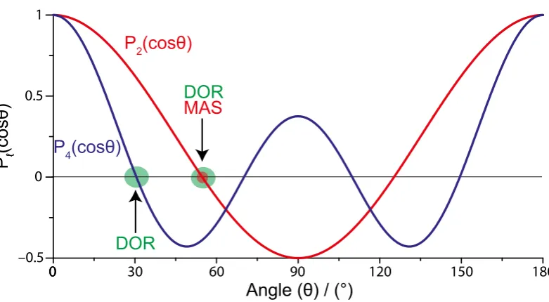
[image:31.595.132.523.105.320.2]

0

Figure 2.2: The Legendre polynomials for l = 2 and 4. The roots from the magic angle is labeled in red (≈54.74o) whilst the roots used in double rotation are labeled in green (≈54.74o and ≈30.56o). This diagram is adapted from Nathan Barrows thesis. [44]

Heredl_m0_m is the reduced rotation matrix which is solely dependent onβ and its products are usually referenced from previous calculations. In a typical NMR experimentm=m0= 0, meaning the reduced Wigner matrix is proportional to the Legendre polynomials by: [45]

Dl₀₀(β) =Pl[cos(β)] (2.10) The angleβ (described from here on as (θ)) describes the angle between the frames after transformations. The terms of interest are the relationship between the LAB frame (static magnetic field, B0) and the PAS frame. The terms of l, of

interest during an NMR experiment, are given below:

P0cos(θ) = 1 (2.11)

P2cos(θ) =

1 2(3 cos

2₍_θ₎₋₁₎ _(2.12)

P4cos(θ) =

1 8(35 cos

4₍_θ₎₋_{30 cos}2₍_θ₎₋₁₎ _(2.13)

(32)

equations are shown in figure 2.2.

The coupling Hamiltonians between a nuclear spin and a magnetic field or other spins can be expressed as a contraction of two second rank Cartesian tensors:

ˆ

H = X

k,l=1,2,3

UklVkl (2.14)

Where U and V are the second rank Cartesian tensors. From the above equations it has been observed thatHˆ is a rank 0 tensor.

Vkl=V0δkl+Vkla+Vkls (2.15) which when substituted into equation 2.14 gives:

ˆ

H = 3U0V0+ X

k,l=1,2,3

U_klaV_kla+U_klsV_kls (2.16)

The above equation is decomposed in terms of isotropic, symmetric and antisymmetric rank 2 Cartesian tensors. The process of summing over the indices effectively averages out and eliminates the cross terms between the symmetry types. This can be done by inverting the zero, first and second rank spherical tensors and substituting them back into the above equation.

The determined rank tensors are given, from zero to second order, as: [41]

T00=V0 (2.17)

T10=V12a, T1±1 =±

1

√

2(V a

23±iV13a) (2.18)

T20=

r

3 2V

s

33, T2±1 =±(T13s ±iT23s) (2.19)

T2±2=

1

2(V11−V22±i2V s

12) (2.20)

Which when substituted into the previous equation becomes:

ˆ

H =

2 X

l=0

(3−l) X

m=l,l−1...l

(−)mTl−m(U)Tlm(V) (2.21)

(33)

ˆ

Hλ ₌_γ

2 X

l=0

(3−l) X

m=l,l−1...l

(−)mTl−m(U)Tlm(V) (2.22)

The corresponding expressions from the chemical shift, dipolar coupling and the quadrupolar interactions are given in the future sections.

2.3.2 Zeeman Interaction

NMR is conducted at a strong magnetic field which has traditionally been defined as the z-axis giving B = (0,0, B0). The Zeeman interaction is shown to quantize

these spins along this vector, IZ =m. With the energy of this interaction defined as the Zeeman Hamiltonian: [46]

ˆ

HZ =−γB0IZ (2.23)

where γ is the previously noted gyromagnetic ratio between the magnetic moment,µ, and the spin angular momentum defined asI.

µ=γI (2.24)

The strength of this interaction is defined by the precession frequency of the nucleus in the static strong magnetic field B0, which is typically five orders of

magnitude higher than the Earth’s magnetic field:

ω0 =−γB0 (2.25)

Where ω0 is the Larmor frequency given in terms of rads−1 and the

gyro-magnetic ratio is measured in rads−1T−1 and the static magnetic field is usually expressed in Tesla (T). Without this strong magnetic field then the spin-up and spin-down states would be degenerate, hence the magnetic field is required to break this degeneracy by a difference ofω0.

Each NMR active isotope’s nucleus has a different Larmor frequency since each magnetic moments differ, this allows an NMR experiment to view differing isotopes, which makes the technique a valuable tool in the analysis of materials. However, each isotope’s receptivity (Γ) is proportional to its gyromagnetic ratio, its nuclear spin (I) and its natural abundance (N A).

Γ =γ3×N A×I(I+ 1) (2.26)

(34)

Magnetic Field (B₀)

1_{H (}_I₌1_/

2) 15N (I = 1/2) 27Al (I = 5/2)

Energy

Magnetic Field (B₀) Magnetic Field (B₀)

E_-5/2 = -5_/ 2γħB0

E_-3/2 = -3_/ 2γħB0

E-1/2 = -1/2γħB0

E_1/2 = 1_/ 2γħB0

E_3/2 = 3_/ 2γħB0

E_5/2 = 5_/ 2γħB0

E_-1/2 = -1_/ 2γħB0

E_1/2 = 1_/ 2γħB0

E_-1/2 = -1_/ 2γħB0

ω₀

0 0 0

ω₀ _ω

0

ω₀ ω₀

ω₀

[image:34.595.128.530.106.365.2]

ω₀

Figure 2.3: The proportional Zeeman splitting for the nuclei1H,15N and 27Al in an arbitrary incremented magnetic field. Adapted from reference [46]

typically referenced to proton or the significantly less receptive13C nucleus (0.00017 with respect to 1.00 for the proton nucleus).

2.3.3 Indirect Dipole - Dipole Coupling

The indirect dipole - dipole coupling is often referred to as the J-coupling, scalar coupling or spin-spin coupling. J-coupling is the indirect through bond coupling of two nuclear spins caused by the influence on the system’s electrons inside a magnetic field. Nuclear spins can interact via their neighbouring electrons to perturb the Hamiltonian of a local through space nuclear spin. [47]

The full Hamiltonian for the J-coupling term between two spins labeled I

andS is given as:

ˆ

(35)

theJIS term is averaged to its isotropic form making theJ-coupling a scalar which is equal to its average diagonal elements: [46, 48]

JIS =

1

3(Jxx+Jyy+Jzz) (2.28) The anisotropic part of the J-coupling tensor has the same form as the dipolar coupling interaction, however it is usually smaller making deconvolution of the interactions very difficult. For the purpose of this thesis the J-coupling interactions (isotropic and anisotropic) tend to be so small they are ignored.

2.3.4 Dipolar Coupling

The dipolar coupling is heavily used in NMR as it can be used to give distance information between spins. This has been universally explained by the analogue of two bar magnets near each other, when you move one the other tries to correct itself to minimise the energy. It is possible to describe this in a classical expression which can be combined with the quantum mechanical magnetic moment (µ) to produce the dipolar Hamiltonian displayed below: [49]

ˆ

HD =−

µ0

4π

¯

hγIγS

r3 Iˆ·Sˆ−

3( ˆI·r)( ˆS·r)

r2

!

(2.29)

Here the gyromagnetic ratios of the two spin systemI and Sare represented by γI and γS respectively. The ’strength’ of this interaction is dependent on the distance between the two spins, hence it is possible to determine the distance be-tween two spins if the dipolar coupling terms can be isolated. To complete this a dipole-dipole coupling (bjk) constant, between two spins j and k, is required to be defined.

bjk =−

µ0

4π

¯

hγIγS

r3 (2.30)

When converted into the PAS frame, the spatial term does not commute to zero, leaving the following Hamiltonian:

ˆ

HP AS

D =AP AS20 Tˆ20P AS (2.31)

Here the spatial term is proportional to:

(36)

ˆ

T₂₀P AS = √1

6(3 ˆIZ ˆ

SZ−IˆZ·SˆZ) (2.33) When rotated into the LAB frame using a single rotation matrix (D2₀₀), which creates the Legendre polynomial, the final dipolar Hamiltonian becomes:

ˆ

HLAB

D =bjk

1 2(3 cos

2_θ₋_{1)(3 ˆ}_I

ZSˆZ−IˆZ·SˆZ) (2.34) In the above equation θ (see figure 2.7) is the angle between the two spins which may vary between 0 andπ. Early experiments on well isolated spins showed that the angular dependence would produce aPake doublet. [50] However, systems with large numbers of interacting spins the end result is usually broadened into a Gaussian/Lorentzian peak. Due to the size of this interaction being comparatively small when observed next the discussed quadrupole and chemical shift components this interaction is not present in any results in this thesis.

2.3.5 Chemical Shift

NMR is a widely used technique today due to the ability to detect differing nuclear environments. This was named the chemical shielding and indicates that the exact resonance frequency is sensitive to the chemical environment around a studied nu-cleus. Chemical shielding is down to a change in the local magnetic field around the nuclei studied, as electrons around these centres produce local magnetic fields. The chemical shift Hamiltonian is best described by: [51]

ˆ

HCS =−γ¯hI·δB0 (2.35)

where·δis the chemical shift tensor. The chemical shielding tensor is given as

σ (δ=−σ). It should be noted that the magnetic shielding (σ) is a tensor property as it depends on the orientation of the molecule with respect to the magnetic field. This becomes apparent during the rotation of a single crystal during a NMR ex-periment. The magnetic shielding tensor describes the change in magnetic field due to the interaction of the neighbouring electrons with B0. This change can produce

shielding or deshielding at the nuclear site as the local magnetic field is increased and decreased respectively. This means that the shielding tensor is referenced to the bare nucleus of atom.

(37)

and calculated directly and hence all calculations of shifts are taken by converting the shielding to the shift via a known standard (see Density Functional Theory sec-tion for more on this). From the Internasec-tional Union of Pure and Applied Chemistry (IUPAC) guidelines the relationship between the chemical shift and the magnetic shielding is given as: [52]

δi=

(σref −σi) (1−σref)

(2.36)

The references selected in the IUPAC guidelines take into consideration the paramagnetic contribution to the magnetic shielding as well as the molecules centre of mass.

The chemical shift is a second-rank tensor quantity which experimentally is given as a real symmetric 3 x 3 matrix.

  

δxx δxy δxz

δxy δyy δyz

δxz δyz δzz

 

 (2.37)

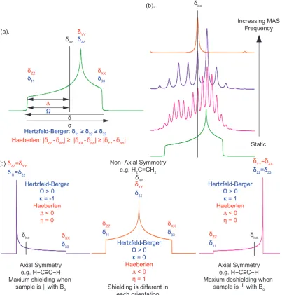
The observable part of the shift tensor is symmetric withδij = δji, the six parameters can be measured per observed nucleus. It is experimentally difficult to achieve this due to lack of resolution and the only recorded data of this type in the literature takes place on very large single crystals with established diffraction data. Hence, the emphasis is usually put on the diagonalized form of the tensor equation and the three values that can be measured in powder line shapes are as follows: [53]

  

δ11 0 0

0 δ22 0

0 0 δ33  

 (2.38)

The three non-zero components of the matrix (the principal components) are defined in a Haeberlen-Mehring-Speiss convention such thatδ11≥δ22≥δ33. These

components represent the shielding in three orthogonal directions of a Cartesian coordinate system. The orientations of the shielding components with respect to the molecule are lost in the diagonalisation process, therefore the values are ordered serially. In a NMR experiment the δ11 component of the line represents the least

shielded resonances, whilst the δ33 parameter is the most shielded. The isotropic

(38)

discussed in this format (IUPAC, δ11, δ22, δ33) and will be presented in the results

as the IUPAC, Haeberlen and Hertzfeld-Berger methods derived below.

In the Herzfeld-Berger notation, a tensor is described by three parameters, which are combinations of the principal components in the standard notation. The first is the isotropic value, which is as previously discussed, the centre of gravity of the resonance. The span (Ω) describes the maximum width of the powder pattern and finally the skew (κ) of the tensor is a measure of the degree of the asymmetry of the tensor. Depending on the position ofδ22 with respect to δiso, the sign is either positive or negative. If δ22 equals δiso, the skew is zero. In the case of an axially symmetric tensor, δ22 equals either δ11 or δ33. Hence, the skew falls with in the

range±1. This method is commonly used by simulation programs (i.e. Quadfit) as it only requires two shifts being known. [54]

δiso =

(δ11+δ22+δ33)

3 (2.39)

Ω = δ11−δ33, Ω>0, formally =

δ11−δ33

1−σref

(2.40)

κ = 3(δ22−δiso)

Ω , 1≤κ≤ −1 (2.41)

The Haeberlen convention uses different combinations of the principal com-ponents to describe the line shape. This convention requires that the principal components are ordered according to their separation from the isotropic value. The centre of gravity of the line shape as previously described by the isotropic value, which is the average value of the principal components. The anisotropy and re-duced anisotropy describe the largest separation from the centre of gravity. The sign of the anisotropy indicates on which side of the isotropic value one can find the largest separation. The asymmetry parameter indicates by how much the line shape deviates from that of an axially symmetric tensor. In the case of an axially symmetric tensor, ∆δ= (δY Y −δXX) will be zero and hence η= 0. [55]

(δ11+δ22+δ33)

3 (2.43)

Reduced Anisotropy, δ = δZZ−δiso (2.44) Anisotropy, ∆δ = δZZ −(δXX+δY Y)

2 , =

3δ

2 (2.45)

(39)

δ11=δ22

δZZ=δYY

δ₃₃

δ_XX

δ₂₂=δ₃₃

δYY=δXX

δ₃₃ δ_XX δ11 δZZ δ₁₁ δ_ZZ δ₂₂ δ_YY δiso δiso δ₁₁ δ_ZZ δ₃₃ δ_XX δ₂₂ δ_YY ∆ Ω δ σ

[image:39.595.125.529.168.590.2]

Hertzfeld-Berger: δ₁₁ ≥ δ₂₂ ≥ δ₃₃

Frequency

Hertzfeld-Berger

Ω > 0 κ = -1 Haeberlen

∆ < 0 η = 0

Hertzfeld-Berger

Ω > 0 κ = 1 Haeberlen

∆ < 0 η = 0

δ_iso δ_iso

δ_iso

(a).

(b).

(c).

Hertzfeld-Berger

Ω > 0 κ = 0 Haeberlen

∆ < 0 η = 1

Axial Symmetry

e.g. H−C≡C−H

Maxium shielding when sample is || with B0

Axial Symmetry

e.g. H−C≡C−H

Maxium deshielding when

sample is ┴ with B0 Non- Axial Symmetry

e.g. H₂C=CH₂

Shielding is different in each orientation

(40)

The previous conventions have been summarised in diagrammatic format in figure 2.4.

2.3.6 Quadrupole Interaction

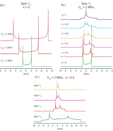
Over two-thirds of the nuclei present in the Periodic Table are quadrupole, meaning they contain a non-spherical nucleus which produces electric quadrupole moment. The coupling of this quadrupole moment to its surrounding electric field gradient is known as the quadrupole interaction.

If a quadrupole nucleus is considered in free space, wherex,y andz axis are equivalent then the Hamiltonian is as follows: [43]

¯

hHˆQ=

eQ

6I(2I−1)

X

j,k=x,y,z

Vjk

3

2(IjIk+IkIj)−δjkI(I+ 1)

(2.47)

HereVjkare the Cartesian components of EFG (V) at the nuclear site, which is given as a second-rank symmetrical tensor. Ij is operator of theJ-component of the spin,I is the spin quantum number,δjk is the Kronecker delta. [56]2

V=

  

VXX 0 0

0 VY Y 0 0 0 VZZ

 

 (2.48)

where

|VZZ| ≥ |VY Y| ≥ |VXX| (2.49)

The Laplace equation (∇2_ϕ _{= 0) still holds true for} _V _{such that} _V

XX +

VY Y +VZZ = 0 as the electric field gradient produced by the nucleus is generated by external nuclear charges. This means only two independent parameters remain theeq and theη, which are given as: [57]

eq=VZZ (2.50)

2

(41)

10 6 4 2 0 (kHz)

-2 -4 -6 -8 -10

8 10 6 4 2 0

(kHz)

-2 -4 -6 -8 -10 8

10 6 4 2 0

(kHz)

-2 -4 -6 -8 -10 -12 8

Spin 3_/ 2 Spin 5_/

2 Spin 7_/

2 Spin 9_/

2

C_Q = 2 MHz, η = 0.5

Spin 5_/

2

η = 0

C_Q = 2 MHz C_Q = 3 MHz C_Q = 4 MHz

Spin 5_/

2

C_Q = 2 MHz

η = 0 η = 0.2 η = 0.4 η = 0.6 η = 0.8 η = 1

(a.)

(c.)

[image:41.595.133.524.156.611.2]

(b.)

(42)

ηQ =

VXX−VY Y

VZZ

, 1≥η ≥0 (2.51)

As VZZ is the largest component of V then this only needs to be consid-ered when addressing eq. In static powder lineshapes obtained during the NMR experiment,eqdescribes the width of the line in MHz and ηgives the characteristic quadrupolar line shape produced. From this the quadrupolar coupling constant can be arrived at by dividing by Planck’s constant, as shown below:

Cq= e

2_qQ

h (2.52)

When moving from the principal axis system (PAS), with respect to V the quadrupole interaction takes the form: [58]

¯

hHˆQ=

e2qQ

4I(2I−1)

3I_Z2 −I(I+ 1) +η(I_X2 −I_Y2) (2.53) If the quadrupole interaction of the above proposed free nucleus is now trans-ferred from Cartesian tensor space into a second-rank irreducible spherical tensor then a simplified representation is observed.

ˆ

HQ=

eQ

2I(2I−1)¯h 2 X

q=−2

(−1)qV(2,−q)T(2,q) (2.54)

also used in the literature is:

ˆ

HQ =

r

3 2

eQ

2I(2I−1)¯h 2 X

q=−2

(−1)qA(2,−q)T(2,q) (2.55)

(43)

V₍₂_,₀₎ =

√

6

2 VZZ (2.56)

V(2,1) = −VXZ−iVY Z (2.57)

V(2,−1) = VXZ−iVY Z (2.58)

V(2,2) =

1

2(VXX−VY Y) +iVXY (2.59)

V₍₂_,−2) =

1

2(VXX−VY Y) +iVXY (2.60)

T(2,0) =

√

6 6

3I_Z2 −I(I+ 1) (2.61)

T(2,1) = −1

2(IZI++I+IZ) =− 1

2I+(2IZ+ 1) (2.62)

T(2,−1) = 1

2(IZI−+I−IZ) = 1

2I−(2IZ−1) (2.63)

T(2,2) = 1

2I+2 (2.64)

T(2,−2) = 1 2I

2

− (2.65)

With these considerations the spherical tensor representation of the quadrupole interaction equation becomes:

ˆ

HQ =

eQ

2I(2I−1)¯h √

6 6 [3I

2

Z−I(I+ 1)]V(2,0)+

1

2I+(2IZ+ 1)V(2,1)

−1

2I−(2IZ−1)V(2,1)+ 1 2I

2

+V(2,−2)+

1 2I

2

−V(2,2) (2.66)

If this result is expressed in terms of the PAS Hamiltonian of the EFG tensor along with equations determined for V and T, then the following spherical tensor components can be revealed. [58]

V₍₂P AS_,₀₎ =

r

3

2eq (2.67)

V₍₂P AS_,_±₁₎ = 0 (2.68)

V₍₂P AS_,_±₂₎ = 1

2eqη (2.69)

(44)

As previously commented, a nuclear spin possesses a magnetic momentµand an angular momentum ¯hI. These fundamental parameters are related by the gyro-magnetic ratioγ. In the LAB frame the coupling of this magnetic moment withB0

is known and previously stated as the Zeeman interaction. The quadrupole Hamilto-nian ( ˆHQ) can be treated as a weak perturbation on this Zeeman interaction( ˆHZ). For this process to take place it is convenient to make the subject time-dependent which requires converting from the LAB frame to the rotating (OBS) frame.

¯

hHˆQ(t) = exp(iHˆZt)¯hHˆQexp(−iHˆZt) (2.70)

= eQ

4I(2I−1)

1 3

√

6[3 ˆI_Z2 −I(I+ 1)]V0

+ Î+(2 ÎZ+ 1)V−1exp(−iω0t)−Iˆ−(2 ÎZ−1)V1exp(iω0t)

+ ˆI₊2V−2exp(−i2ω0t) + ˆI−2V2exp(i2ω0t) (2.71)

The secular term remains time-independent and in order to make the equa-tion completely time-independent,HˆQ(t) is averaged over one Larmor period (2_ωπ₀) up to the first order.

D

ˆ

HQ(t)

E

= ω0 2π

Z 2π ω₀

0

dtHˆQ(t)−

iω0

4π Z 2π

ω₀

0 dt

Z t 0

dt0[ ˆHQ(t),HˆQ(t0)] (2.72)

= Hˆ_Q(0)+H_Q(1) (2.73)

As only the secular terms commute with IZ and with some simplification ˆ

H(0)

Q and Hˆ

(1)

Q can be considered as the first ( ˆH

[1]

Q ) and the second ( ˆH

[2]

Q ) order quadrupole terms.

ˆ

H[1]

Q =Hˆ

(0)

Q =

eQ

4I(2I−1)¯h √

6 3 [3I

2

Z−I(I + 1)]V0 (2.74)

ˆ

H[2]

Q =Hˆ

(1)

Q =−

1

ω0

eQ

4I(2I−1)¯h 2

×(2V−1V1IZ[4I(I+ 1)−8IZ2 −1]

+ 2V−2V2IZ[2I(I+ 1)−2IZ2 −1]) (2.75)

(45)

rotat-ing frame to the laboratory frame, as they both commute withIZ. A more obvious point to note is thatHˆ_Q[1] is independent ofω0, whilstHˆ_Q[2] is inversely proportional

to ω0, therefore at higher magnetic fields there is a reduction in the second order

quadrupole term.

The energy levels (2I+1) of a free spinIwhen introduced to a static magnetic field, creating the Zeeman interaction, are defined as Dm

ˆ HZ m E

= −mω0 with

the difference between two neighbouring energy levels (m−1, m) given with respect to angular velocity as:

ω_m(Z₋)₁_,m=

D

m−1

HˆZ

m−1

E −Dm

HˆZ

m

E

=ω0 (2.76)

From this basis the first order quadrupole interaction shifts the energy levels by an amount proportional to

D m ˆ H[1] Z m E = eQ

4I(2I−1)¯h √

6 3 [3m

2₋₁₍_I _{+ 1)]}_V

0 (2.77)

With the contribution of the line position associated with the transition of

m−1, mbeing equal to

ω_m(1)₋₁_,m =

D

m−1

Hˆ [1] Z m−1

E −Dm

H [1] Z m E (2.78)

= 3eQ 4I(2I−1)¯h

√

6

3 (1−2m)V0 (2.79)

The spectrum conceived from this equation gives 2Ilines, a central transition which is represented by the−1

2, 1

2 transitions which is located atω0, with the other

2I−1 representing the satellite resonances.

The following line is shifted further when you take into consideration the second order quadrupole interaction: [60]

ˆ

H[2]

Q =Hˆ

(1)

Q =−

1

ω0

eQ

4I(2I−1)¯h 2

×(2V−1V1m[4I(I+ 1)−8m2−1]

+ 2V−2V2m[2I(I+ 1)−2m2−1]) (2.80)

(46)

ω_m(2)₋₁_,m=

D

m−1

ˆ H[2] Z m−1

E −Dm

ˆ H[2] Z m E (2.81)

=− 2

ω0

eQ

4I(2I−1)¯h 2

×(V−1V1[24m(m−1)−4I(I+ 1) + 9]

+1

2V−2V2[12m(m−1)−4I(I+ 1) + 6]) (2.82) Thus the associated contribution of the first and second order quadrupole interaction is given as:

ωm−1,m=ω0+ω(1)m−1,m+ω

(2)

m−1,m (2.83) In order to produce an equation representative of a static NMR resonance it is required to express theV0terms of the aboveω(1)m−1,mequation and theV1, V−1, V2

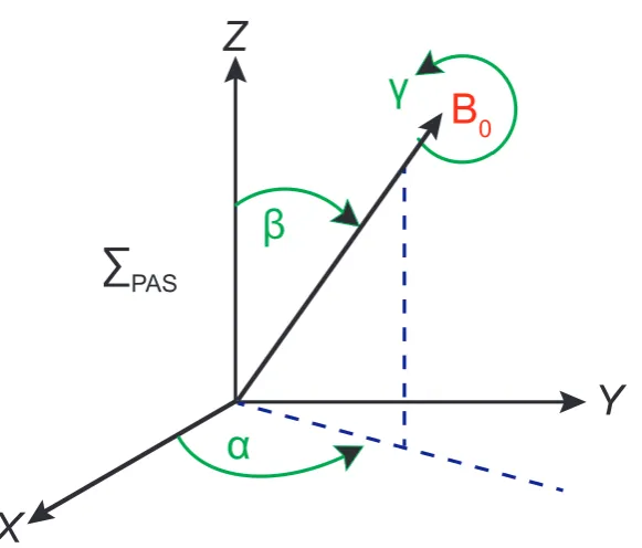
and V−2 terms of the ω_m(2)−1,m derivation in the terms of V in the principal axis system. Thus, it is required to define the Euler angles in a strong static magnetic field.

Vi=

2 X

j=−2

D(2)_j,i(α, β, γ)V_JP AS (2.84)

Here the Euler angles (α, β and γ) describe the direction in the magnetic field (PP AS_). _D

j,i is the Wigner rotation matrix defined in the following diagram (see figure 2.6). [61]

Therefore,V0 is given as:

V0 =

r

3 2eq[

1 2(3 cos

2_β₋_{1) +} 1

2ηsin

2_β_{cos 2}_α_] _(2.85)

When this equation is substituted into equation 2.74 yields:

ˆ

H[1]

Q =

1 3ωQ[3I

2

Z−I(I+ 1)] (2.86) with:

ωQ=

3χ

4I(2I−1)[ 1 2(3 cos

2_β₋_{1) +} 1

2ηsin

(47)

X

Z

Y

B

₀

α

β

∑

_PAS

[image:47.595.178.469.106.354.2]

γ

Figure 2.6: The Euler angles defining the direction of B0 in the PAS of the EFG

during a static NMR experiment

Depending on the Euler angle convention used a negative sign can be substi-tuted in front of the η parameter. When reproduced to take into consideration the first order quadrupolar shift of the line as in equation 2.78. [25]

ω(1)_m₋Static₁_,m = (1−2m)ωQ (2.88)

The lines in the spectrum will become shifted by the same quantity (2ωQ) with the central line not being shifted.

The other two factors deduced from equation 2.82 are:

2V1V−2=−

3 2e

2_q2_[(₋1

3η

2_cos2₂_α_{+ 2}_η_{cos 2}_α₋_{3) cos}4_β

+ (2 3η

2_cos2₂_α₋₂_η_{cos 2}_α₋1

3η

2_{+ 3) cos}2_β

+1 3η

(48)

V2V−2=−

3 2e

2_q2_[( 1

24η

2_cos2₂_α₋1

4ηcos 2α+ 3 8) cos

4_β

+ (− 1

12η

2_cos2₂_α₊1

6η− 3 3η

2_{+ 3) cos}2_β

+ 1 24cos

2₂_α₊1

4ηcos 2α+ 3

8] (2.90)

The second order quadrupole shift of the central line is derived from equation 2.82 giving:

ω(2)₋₁_/Static₂_,₁_/₂ =− 1

6ω0

3χ

2I(2I−1)

2

[I(I+ 1)−3

4]

×[A(α, η) cos4β+B(α, η) cos2β+C(α, η)] (2.91)

Here:

A(α, η) =−27

8 + 9

4ηcos 2α− 3

8(ηcos 2α)

2 _(2.92)

B(α, η) = 30

8 − 1 2η

2₋₂_η_{cos 2}_α₊ 3

4(ηcos 2α)

2 _(2.93)

C(α, η) =−3

8+ 1 3η

2₋1

4ηcos 2α− 3

8(ηcos 2α)

2 _(2.94)

When the EFG has axial symmetry atη= 0 then the equation simply reduces to:

ω(2)₋₁_/Static₂_,₁_/₂ =− 1

16ω0

3χ

2I(2I−1)

2

[I(I+ 1)− 3

4]

×(1−cos2β)(9 cos2β−1) (2.95)

It is worth noting that the Euler angle γ is not present in any of the above equations, this is becauseB0 is the symmetry axis for the spins. Wolf and co-workers

have shown that the third order term is proportional to 2m_ω−21 0

, hence the line is not shifted further by the addition of this perturbation. [62]

2.3.7 The Knight Shift

The Knight shift, named after its discoverer Walter David Knight, is the relative shift

(49)

to the absolute temperature. In superconductors (at operational temperatures) the shift decreases dramatically as the electron spins pair up to form spin-pair bosons. This is a primary characteristic of a superconducting state. [22]3

As conduction electrons in a metal are not uniquely associated with any par-ticular nucleus more than another then they all exist within eigenstates known as a band. The highest occupied state of this band is known as the Fermi energy,Ef at T = 0K. Close to Ef the electron wavefunctions tend to be dominated by mixtures ofp and d orbitals whilst at lower energies the s states are more prevalent. Thes -electrons at the nuclear site have a high probability density (R= 0), as each electron contains spin and charge this in turn causes an interaction which produces a local magnetic field. Hence, the Knight shift is caused by the non-localised conduction electrons effectively producing additional shielding at the nuclear site. The con-duction electron states occupy a Fermi distribution and due to the Pauli exclusion principle they become occupied pairwise: meaning every energy level will contain a spin up and spin down electron. When a magnetic field is applied, there is an imbalance in this spin up and down distribution causing the Pauli susceptibility and a net magnetization giving a shift in the resonance. The observed shielding term is the sum of the chemical shift and the induced Knight shift (K) and as they both scale with field it becomes difficult to separate the components. The total shift of the line is hence described as a percentage of the field: [48]

T otal Shif t=Ks+Kd+Kcp+σ=K+σ (2.96)

Where Ks represents thes-electron contribution to the shift and Kd gives thed-electron involvement, these both give a positive shift as seen in tin metal. If the hyperfine fields of the conductions-electrons induce a polarisation in the inner core s-electrons then a subsequent shift can be produced, this is termed the core polarisation Kcp. This gives a negative shift as seen in platinum metal. In a two band model of a simple spherical platinum nanoparticle, the contribution from the platinum 5dband is shown to be negative whilst those from the 6sband is positive, the relaxation is proportional to a sum of the squares (i.e. Ki2) and is therefore always positive. The d-electron contribution is shown to decay exponentially from bulk metal as you move upfield towards the platinum 001 surface. This is discussed at far greater length in the platinum PEM catalyst chapter. [63]

The Knight shift is typically expressed as a percentage with respect to the primary IUPAC reference used for the chemical shift ranges. The limitations of this

3