Least Squares Method from the View Point of Deep Learning II: Generalization

(1)

ISSN Online: 2160-0384 ISSN Print: 2160-0368

DOI: 10.4236/apm.2018.89048 Sep. 25, 2018 782 Advances in Pure Mathematics

Least Squares Method from the View Point of

Deep Learning II: Generalization

Kazuyuki Fujii

1,2

1_{International College of Arts and Sciences, Yokohama City University, Yokohama, Japan} 2_{Department of Mathematical Sciences, Shibaura Institute of Technology, Saitama, Japan}

Abstract

The least squares method is one of the most fundamental methods in Statis-tics to estimate correlations among various data. On the other hand, Deep Learning is the heart of Artificial Intelligence and it is a learning method based on the least squares method, in which a parameter called learning rate plays an important role. It is in general very hard to determine its value. In this paper we generalize the preceding paper [K. Fujii: Least squares method from the view point of Deep Learning: Advances in Pure Mathematics, 8, 485-493, 2018] and give an admissible value of the learning rate, which is eas-ily obtained.

Keywords

Least Squares Method, Statistics, Deep Learning, Learning Rate, Gerschgorin’s Theorem

1. Introduction

This paper is a sequel to the preceding paper [1].

The least squares method in Statistics plays an important role in almost all disciplines, from Natural Science to Social Science. When we want to find properties, tendencies or correlations hidden in huge and complicated data we usually employ the method. See for example [2].

On the other hand, Deep Learning is the heart of Artificial Intelligence and will become a most important field in Data Science in the near future. As to Deep Learning see for example [3]-[10].

Deep Learning may be stated as a successive learning method based on the least squares method. Therefore, to reconsider it from the view point of Deep Learning is natural and instructive. We carry out the calculation thoroughly of How to cite this paper: Fujii, K. (2018)

Least Squares Method from the View Point of Deep Learning II: Generalization. Ad-vances in Pure Mathematics, 8, 782-791.

https://doi.org/10.4236/apm.2018.89048 Received: August 30, 2018

Accepted: September 22, 2018 Published: September 25, 2018 Copyright © 2018 by author and Scientific Research Publishing Inc. This work is licensed under the Creative Commons Attribution International License (CC BY 4.0).

(2)

DOI: 10.4236/apm.2018.89048 783 Advances in Pure Mathematics the successive approximation called gradient descent sequence, in which a parameter  called learning rate plays an important role.

One of main points is to determine the range of the learning rate, which is a very hard problem [8]. We showed in [1] that a difference in methods between Statistics and Deep Learning leads to different results when the learning rate changes.

We generalize the preceding results to the case of the least squares method by polynomial approximation. Our results may give a new insight to both Statistics and Data Science.

2. Least Squares Method

Let us explain the least squares method by polynomial approximation [9]. The model function f x

( )

is a polynomial in x of degree M given by

( )

0 1

0 .

M

M j

j f x w w x w x w x

=

= + + + =

∑

(1) For N pieces of two dimensional real data

(

) (

)

(

)

{

x y1, 1 , x y2, 2 , , x yN, N

}

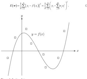
we assume that their scatter plot is given like Figure 1.

The coefficients of (1)

(

)

T

0, , ,1 M w w w =

w  ₍₂₎ must be determined by the data set (T denotes the transposition of a vector or a matrix).

For this set of data the error function is given by

( )

{

( )

}

2 2

1 1 0

1 1 _.

2 2

N N M

j

i i i j i

i i j

E y f x y w x

= = =

 

= − =  − 

 

∑

w

[image:2.595.239.532.451.718.2]

(3)

DOI: 10.4236/apm.2018.89048 784 Advances in Pure Mathematics The aim of least squares method is to minimize the error function (3) with respect to

w

in (2). Usually it is obtained by solving the simultaneous differentiable equations

( )

0

1

0,

0. M E

w E

w

E w ∂

=  ∂  ∂

 =

 _∂    ∂

= 

∂ 

w

w 

However, in this paper another approach based on quadratic form is given, which is instructive.

Let us calculate the error function (3). By using the definition of inner product

T

1 1 2 2 n n

a b a b a b

= + + + =

a b  a b

it is not difficult to see

( )

2E w = y− Φw y− Φw

₍₄₎

where

(

)

T

(

)

T

1, , ,2 N , 0, , ,1 M

y y y w w w

= =

y  w 

and

1 2

1 1 1

1 2

2 2 2

1 2 1

1 _.

1

M

N N N

x x x

 

 

Φ =  

 

 

 

    

 Here we make an important

Assumption N M> +1 and rank

( )

Φ =M +1 (full rank). Let us deform (4). From

(

) (

)

(

)

(

)

(

)

(

)

T

T T T

T T T T T T

− Φ − Φ = − Φ − Φ

= − Φ − Φ

= Φ − Φ −

= Φ Φ − Φ − Φ +

y w y w y w y w

y w y w

w y w y

w w w y y w y y we set for simplicity

T T T

, A , , c .

= = Φ Φ = Φ =

x w b y y y

Namely, we have a general quadratic form

( )

T T T

2E w = y− Φw y− Φw =x x x b b xA − − +c.₍₅₎ On the other hand, the deformation of (5) is well-known.

Formula For a symmetric and invertible matrix A (:_∃_A−1_{) we have}

(

) (

T

)

T_A ₋ T ₋ T _{+ =}_c ₋_A−1 _A ₋_A−1 ₋ T_A−1 ₊_c_.

x x x b b x x b x b b b

(4)

DOI: 10.4236/apm.2018.89048 785 Advances in Pure Mathematics The proof is easy. Since _AT_{= ⇒}_A

( )

_A−1 T₌_A−1_{we obtain}

(

₁

) (

T ₁

) (

_T _T ₁

) (

₁

)

T T T T 1

A A A A A A

A A

− − − −

−

− − = − −

= − − +

x b x b x b x b

x x x b b x b b and this gives (6).

Therefore, our case becomes

( )

{

(

)

}

{

(

)

}

(

)

T

1 1

T T T T T

1

T T T T

2E − −

−

= − Φ Φ Φ Φ Φ − Φ Φ Φ

− Φ Φ Φ Φ +

w w y w y

y y y y

(7)

because _{Φ Φ}T _{is symmetric and invertible by the assumption.} If we choose

(

_T

)

−1 _T

= Φ Φ Φ

w y

(8) then the minimum is given by

( )

_T _T

(

_T

)

1 _T _T

{

(

_T

)

1 _T

}

min

2E EN

− −

= − Φ Φ Φ Φ = − Φ Φ Φ Φ

w y y y y y y

(9) where EN is the N-dimensional identity matrix.

Our method is simple and clear (“smart” in our terminology).

3. Least Squares Method from Deep Learning

In this section we reconsider the least squares method in Section 2 from the view point of Deep Learning.

First we arrange the data in Section 2 like

(

)

{

2

}

Input data : 1, , , , M |1

j j j

x x  x ≤ ≤j N

{

1 2

}

Teacher signal : y y, , , yN

and consider a simple neuron model in [11] (see Figure 2).

Here we use the polynomial (1) instead of the sigmoid function z=σ

( )

x . In this case the square error function becomes

( )

1 1

(

T T T T T T

)

_.

2 2

L w = y− Φw y− Φw = w Φ Φ −w w Φ y y w y y− Φ +

[image:4.595.200.537.66.351.2]

(10)

(5)

DOI: 10.4236/apm.2018.89048 786 Advances in Pure Mathematics We in general use L

( )

w instead of E

( )

w in (3).

Our aim is also to determine the parameters

w

in order to minimize L

( )

w . However, the procedure is different from the least squares method in Section 2. This is an important and interesting point.

The parameters

w

are determined successively by the gradient descent method (see for example [12]): For t=0,1,2,

( )

0 →

( )

1 → →

( )

t →

(

t+ →1

)

w w  w w 

and

(

t 1

)

( )

t L

_{( )}

t ∂

+ = −

∂

w w

w 

(11) where

( )

(

)

1

{

( )

T T

( )

T T T

( )

T

}

2

L L= w t = w t Φ Φw t −w t Φ y y w− Φ t +y y

(12) and 

(

0< < 1

)

is a small parameter called the learning rate.

The initial value w

( )

0 is given appropriately. Pay attention that t is discrete time and T is the transposition.

Let us calculate (11) explicitly. Since

( )

T

( )

T

L _t

t

∂ _{= Φ Φ} _{− Φ}

∂w w y

from (12) we have

(

)

( )

{

T

( )

T

} (

T

)

( )

T

1

1 M .

t+ = t − Φ Φ t − Φ = E + − Φ Φ t + Φ

w w  w y  w  y

(13) This equation is easily solved to be

( )

(

_T

)

( )

{

(

_T

)

}

(

_T

)

1 _T

1 0 1 1

t t

M M M

t = E + − Φ Φ + E + − E + − Φ Φ Φ Φ Φ−

w  w  y

(14) for t=0,1,2,.

The proof is left to readers.

Since this is not a final form let us continue the calculation. From (14) we have

( )

(

_T

)

1 _T

lim

t t

−

→∞w = Φ Φ Φ y

(15) if

(

T

)

1 1

lim_t_→∞ EM+ − Φ Φ = t OM+

(16) where OM+1 is the N-dimensional zero matrix. (15) is just the equation (8) and

it is independent of .

Let us evaluate (14) further. The matrix _{Φ Φ}T _{is positive definite, so all} eigenvalues are positive. This can be shown as follows. Let us consider the eigenvalue equation

(

)

T

_λ

_v _.

Φ Φ =v v ≠0

(6)

DOI: 10.4236/apm.2018.89048 787 Advances in Pure Mathematics

T ₀ _0.

λ

v v =

λ

v v = Φ Φv v = Φ Φ > ⇒ >v v

λ

Therefore we can arrange all eigenvalues like

1 2 M 1 0.

λ λ≥ ≥≥λ ₊ > Since _{Φ Φ}T _{is symmetric, it is diagonalized as}

T _QDQT

Φ Φ = ₍₁₇₎

where Q is an element in O M

(

+1

)

₍_QT₌_Q−1_{) and}_D_{is a diagonal matrix}

1 2 1 . M D λ λ λ ₊       =_ _     

See for example [13].

By substituting (17) into (14) and using the equation

(

)

1

2

T T T

1 1 1 1 1 1 M M M

E Q E D Q Q Q

λ λ λ + + + −    ₋   

− Φ Φ = − =

    −         we finally obtain

Theorem I A general solution to (14) is

( )

(

)

(

)

(

)

( )

(

)

(

)

(

)

1 T 2 1 1 1 2 T T 2 1 1 1 1 ₀ 1 1 1 1 1 . 1 1 t t t M t t t M M

t Q Q

Q Q λ λ λ λ λ λ λ λ λ + + +  ₋     −  =      ₋     _{− −}        − −     + Φ       − −       w w y         (18)

This is our main result.

Next, let us show how to choose the learning rate 

(

0< < 1

)

, which is a very important problem in Deep Learning [7][8].

Let us remember

1 2 M 1 0.

λ λ≥ ≥_≥λ ₊ >

From (16) and (18) the equations

(

T

)

(

)

1 1

lim_t_→∞ EM+ − Φ Φ = t OM+ ⇔lim 1_t_→∞ −λj t=0 for 1≤ ≤j M+1

(7)

(

)

(

)

1 1 0 2 lim 1 n 0

n

x x x

→∞

− < ⇔ < < ⇒ − =

and

1 2 M1 0

λ ≥ λ ≥≥ λ + >

  

we obtain

Theorem II The learning rate  must satisfy an inequality

1

2

0 λ 2 0 .

λ < < ⇔ < <

(20) The greater the value of , the sooner goes the gradient descent (11) so long as the convergence (19) is guaranteed. Let us note that the choice of the initial values w

( )

0 is irrelevant when the convergence condition (20) is satisfied.

Comment For example, if we choose  like

1

2 ₁

λ < <

then we cannot recover (15), which shows a difference in methods between Statistics and Deep Learning.

4. How to Estimate the Learning Rate

How do we calculate λ1? Since

{ }

λ

j are the eigenvalues of the matrix Φ ΦT , they satisfy the equation

( )

j 0, 1 2 M 1 0

F

λ

=

λ λ

≥ ≥≥

λ

+ >

where F

( )

λ is the characteristic polynomial of _{Φ Φ}T _{given by}

( )

T

1 .

M

F

λ

=

λ

E + − Φ Φ

(21) This is abstract, so let us deform (21). For simplicity we write Φ_as

( ) ( ) ( ) ( )

(

)

1 2

1 1 1

1 2

0 1 2

2 2 2

1 2 1

1 _, _, _{, ,} _.

1

M

N N N

x x x

 

 

Φ =_ _≡

 

 

x x x x



 _

    



(22)

Then it is easy to see

( ) ( )

(

)

( ) ( )

T

0 , , ₁

N

i j i j i j

k

i j M _k x

+

≤ ≤ ₌

Φ Φ = x x x x =

∑

where the notation a b is the (real) inner product of vectors. For clarity let us write down (21) explicitly.

( )

( ) ( ) ( ) ( ) ( ) ( )

0 0 0 1 0

1 0 1 1 1

0 1

. M M

M M M M

F λ

λ λ

λ

− − −

=

− − −

x x x x x x

x x x x x x

x x x x x x

 

   



(8)

( )

0

F λ = if M is very large1_{. Therefore, let us get satisfied by obtaining an}

approximate value which is both greater than λ1 and easy to calculate.

For the purpose the Gerschgorin’s theorem is very useful2_{. Let}

( )

ij A a= be an

n n

×

_{complex (real in our case) matrix, and we set}

1,

n

i ij

j j i

R a

= ≠

=

∑

(23) and

(

ii; i

)

{

ii i

}

D a R = ∈z C z a− ≤R (24) for each i. This is a closed disc centered at aii with radius Ri called the Gerschgorin’s disc.

Theorem (Gerschgorin [14]) For any eigenvalue λ of A we have

(

)

1 ; .

n

ii i i

D a R

λ

=

∈

_

(25) The proof is simple. See for example [7].

Our case is real and n M= +1 and ( ) ( )

(

)

T

0 , .

i j i j M A

≤ ≤

= Φ Φ = x x

Therefore, all eigenvalues

{ }

λ satisfy

(

)

1

[

]

1 1

; ,

n M

ii i ii i ii i

i i

D a R a R a R

λ +

= =

∈

_

=

_

− +

(26) where

[

A B,

]

is a closed interval and

( )1 ( )1 1 ( )1 ( )1 1,

and M .

i i i i

ii i

k k i

a − − R + − −

= ≠

= x x =

∑

x x

If we define

{

}

1 ₁max₁

M+ = _{≤ ≤ +}_{i M} aii+Ri 

(27) then it is easy to see

1 1

2 _{2 .}

M

M λ

λ

+

≤ ⇒ ≤

 from (26).

Thus we arrive at an admissible value of the learning rate  which is easily obtained.

Theorem III An admissible value of  is

1

2 . M+

= 

 (28) Let us show an example in the case of M =1₍_[1]_{), which is very instructive} for non-experts.

Example In this case it is easy to see and we set

1 _{Φ Φ}T _{is not a sparse matrix.}

(9)

T 1

2

1 1

N i i

N N

i i

N x a x

x X

x x

=

= =

 _{ } _

 

Φ Φ = _{≡ } _

 _{ } _

 

∑

for simplicity. Moreover, we may assume x>0_{. Then from (21) we have}

( )

T 2

(

)

(

2

)

2

f

λ

=

λ

E − Φ Φ =

λ

− a X+

λ

+ aX x−

and

(

)

(

)

(

)

2 2

1

2 2

) 4 2

4 . 2

a X a X aX x

a X a X x

λ = + + + − −

+ + − +

=

On the other hand, from (27) we have

{

}

2=max a x X x+ , +

 because x>0_.

Then it is easy to show

{

}

(

)

2 4 2

max , .

2

a X a X x

a x X x+ + ≥ + + − +

To check this inequality is left to readers. Therefore, from (28) the admissible value becomes

{

2

}

.

max a x X x,

=

+ +



We emphasize once more that M+1 is easy to evaluate, while to calculate λ1

is very hard if M is large.

5. Concluding Remarks

In this paper we have discussed the least squares method by polynomial approximation from the view point of Deep Learning and carried out calculation of the gradient descent thoroughly. A difference in methods between Statistics and Deep Learning delivers different results when the learning rate  is changed. Theorem III is the first result to provide an admissible value of  as far as we know.

Deep Learning plays an essential role in Data Science and maybe in almost all fields of Science. Therefore it is desirable for undergraduates to master it in the early stages. To master it they must study Calculus, Linear Algebra and Statistics from Mathematics. My textbook [7] is recommended.

Acknowledgements

We wishes to thank Ryu Sasaki for useful suggestions and comments.

Conflicts of Interest

(10)

References

[1] Fujii, K. (2018) Least Squares Method from the View Point of Deep Learning. Ad-vances in Pure Mathematics, 8, 485-493.

[2] Wikipedia: Least Squares. https://en.m.wikipedia.org/wiki/Least_Squares [3] Wikipedia: Deep Learning. https://en.m.wikipedia.org/wiki/Deep_Learning [4] Goodfellow, I., Bengio, Y. and Courville, A. (2016) Deep Learning. The MIT Press,

Cambridge.

[5] Patterson, J. and Gibson, A. (2017) Deep Learning: A Practitioner’s Approach, O’Reilly Media, Inc., Sebastopol.

[6] Alpaydin, J. (2014) Introduction to Machine Learning. 3rd Edition, The MIT Press, Cambridge.

[7] Fujii, K. (2018) Introduction to Mathematics for Understanding Deep Learning. Scientific Research Publishing Inc., Wuhan.

[8] Okaya, T. (2015) Deep Learning (In Japanese). Kodansha Ltd., Tokyo.

[9] Nakai, E. (2015) Introduction to Theory of Machine Learning (In Japanese). Gijut-su-Hyouronn Co., Ltd., Tokyo.

[10] Amari, S. (2016) Brain Heart Artificial Intelligence (In Japanese). Kodansha Ltd., Tokyo.

[11] Fujii, K. (2018) Mathematical Reinforcement to the Minibatch of Deep Learning. Advances in Pure Mathematics, 8, 307-320. https://doi.org/10.4236/apm.2018.83016

[12] Wikipedia: Gradient Descent. https://en.m.wikipedia.org/wiki/Gradient_descent [13] Kasahara, K. (2000) Linear Algebra (In Japanese). Saiensu Ltd., Tokyo.