Rational filter design for depth from defocus

University of Warwick institutional repository: http://go.warwick.ac.uk/wrap

This paper is made available online in accordance with

publisher policies. Please scroll down to view the document

itself. Please refer to the repository record for this item and our

policy information available from the repository home page for

further information.

To see the final version of this paper please visit the publisher’s website.

Access to the published version may require a subscription.

Author(s): Alex Noel Joseph Raj and Richard C. Staunton

Article Title: Rational filter design for depth from defocus

Year of publication: 2012

Link to published article:

http://dx.doi.org/10.1016/j.patcog.2011.06.008

Publisher statement: “NOTICE: this is the author’s version of a work

that was accepted for publication in Pattern Recognition. Changes

resulting from the publishing process, such as peer review, editing,

corrections, structural formatting, and other quality control mechanisms

may not be reflected in this document. Changes may have been made

to this work since it was submitted for publication. A definitive version

was subsequently published in Pattern Recognition, VOL:45,

Rational Filter Design for Depth from Defocus

Alex Noel Joseph Raj1 and Richard C. Staunton2

1

School of Engineering, University of Warwick, Coventry CV4 7AL, UK. Email: [email protected]

2

School of Engineering, University of Warwick, Coventry CV4 7AL, UK. Email: [email protected]

Corresponding author: R.C. Staunton. Phone: +44 2476 523980, Fax: +44 2476 418922

This paper was published in the Journal: Pattern Recognition. The full reference is:-

Alex Noel Joseph Raj and Richard C. Staunton, (Jan. 2012) Rational Filters Design for Depth from Defocus. Pattern Recognition, Vol. 45 (No. 1). pp. 198-207.

Abstract

The paper describes a new, simple procedure to determine the rational filters that are used in the depth from defocus (DfD) procedure previously researched by Watanabe and Nayar [4]. Their DfD uses two differently defocused images and the filters accurately model the relative defocus in the images and provide a fast calculation of distance. This paper presents a simple method to determine the filter coefficients by separating the M/P ratio into a linear and a cubic error correction model. The method avoids the previous iterative minimisation technique and computes efficiently. The model has been verified by comparison with the theoretical M/P ratio. The proposed filters have been compared with the previous for frequency response, closeness of fit to M/P, rotational symmetry, and measurement accuracy. Experiments were performed for several defocus conditions. It was observed that the new filters were largely insensitive to object texture and modelled the blur more precisely than the previous. Experiments with real planar images demonstrated a maximum RMS depth error of 1.18% for the proposed, compared to 1.54% for the previous filters. Complicated objects were also accurately measured.

Key Words: Depth from defocus, M/P ratio, Rational filters, 3D imaging.

1. Introduction

[image:3.612.162.451.464.636.2]

processing. DfD is a technique in which the ‘defocus’ at a pixel in an image is used to estimate the distance from the lens to the corresponding point on an object. The method requires two differently focused images acquired from a single view point using a single camera, and the relative blur between the images is used to determine the in-focus axial points of each pixel and hence depth. In this way it differs from the allied method of depth from focus which may use several images [1,2]. Most approaches consider blurring as a linear shift invariant process either in the frequency or spatial domain. The defocused image is modelled as the convolution of the focused image with the point spread function (psf) of the lens [3-8]. The blur information is retrieved by the deconvolution process either in the frequency or spatial domain, and then related to the actual distance using the appropriate depth model. These methods offer an advantage in terms of computation and simplicity in the implementation of the algorithm. An accuracy of 1.2% has been reported from experiments using images of real scenes [4], however it can be difficult to compare the techniques as the accuracy depends on the range over which the measurements were made, with a narrow range close to the camera giving better results. Additionally some researchers use local smoothing operators to remove noise from the final depth map that improve their accuracy figures. Other methods (often statistical) consider the blurring as a shift variant process and retrieve a unique depth value not only along the optical axis but also along the x and y directions of the scene under investigation. These methods can be accurate (1%) and are efficient since they simultaneously retrieve depth and the radiance of the scene, but may not be suitable for practical, real-time, purposes since they are based on error minimisation techniques which require extensive computations [9-14]. Video-rate processing is a requirement for 3D TV, and fast processing extends the use of DfD for robotics and production line applications. Efficient DfD computation methods have been proposed [4,15,16], however in this paper, since we are concerned with video-rate depth estimation for every pixel in the image, and passive illumination, we have chosen an approach based on rational filters [4] as detailed more fully below.

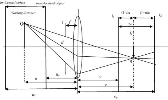
Figure 1. Telecentric DFD system

are 2e apart with if lying in between. Thus on the object side a working range is defined by the lens

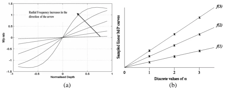
law. Previous DfD methods that were based on the frequency domain approach [3-5] estimated the depth by considering the amplitude ratio of two defocused images at a particular radial frequency. Watanabe and Nayar [4] provided an improvement with the M/P ratio curve set that effectively models the lens defocus performance for particular working conditions at different texture frequencies. They considered the amplitude ratio between the difference (M) of the defocused images to their sum (P), and developed a set of broadband filters that modelled the curves (Figure 2a). Although the filters were designed in the frequency domain, the algorithm was implemented in the spatial domain by employing 2D convolutions. Only 7x7 filter kernels were required and the algorithm enabled the filters to be applied in parallel resulting in efficient hardware implementation. The main advantages of this method were: (1) Higher accuracy in depth estimation. The RMS error reported was 1.2% with respect to distance (which was better than any comparable methods [17]); (2) Invariance to scene texture and illumination (the depth detection error was less than 1% with respective to texture frequency [4]); and (3) The feasibility of high speed calculation using a hardware implementation. Additionally they researched telecentric optics [18] to enable the near and far-focused images to be optically registered by removing the magnification caused by refocusing the lens. In Figure (1) the telecentric aperture is labelled T and is at the front focal point of the lens. We have used telecentric optics with a Phase Correlation technique [19] to measure the radial shifts due to magnification, and also to optimally position the external aperture.

Despite the efficient algorithm, the main drawback of the previous method was the complicated design procedure based on an iterative minimisation technique to model the rational filters for any given defocus condition, and texture frequency. Watanabe [4] has published filter coefficients for the single defocus condition of 2.307 pixels, and subsequent researchers have only published work which used these and no other. In this paper we report a new, simple procedure for rational filter design, the Two Step Polynomial Approach [17]. We have compared our model with Watanabe and Nayar’s, for the defocus condition of 2.307 pixels, for the accuracy with which the filters approximate the M/P ratio curves, and for the overall depth estimation accuracy. For the Two Step Polynomial Approach we have also provided the overall depth estimation accuracy for a range of defocus conditions, using both simulated and real images.

2. Filter design using the Two Step Polynomial Approach

This section describes the new procedure that uses a discrete M/P space and polynomials to determine the filter coefficients that were used in the DfD calculations. Three filters, Gm1, Gp1 and

Gp2 were designed to model the lens defocus M/P ratio curves, and two pre-filters were used to

remove dc (mean) values from the M and P input images. Since the model was based on the M/P ratios, these were calculated for a range of frequencies using the psf of the defocused lens. Various models of the psf exist where an impulse (delta) function can model a perfect lens in focus; a Gaussian function has been used for a lens in near focus [20]; and a pill box (cylindrical) function for a lens that is more defocused [3]. A single generalized Gaussian has been used to model all three regions [21], but to provide a meaningful comparison with Watanabe’s filters [4] their pill box model has been used here. The psf was pre-computed using the Pillbox model for a range of normalized depth values, α from 0 to 0.99. So based on [4], the psf was modelled in the frequency domain using the equation

) ( 2 ) , ; , ( ) ,

( ₁ 2 2

2

2 _F u v

z J v u z F F z v u H v u H e e e + + = = π

π --- (1).

Where, referring to Figure (1),

z

=

(

1

±

α

)

e

denotes the distance between the sensor plane and the focused image if. For a telecentric setup [17,18],

F

_e

=

f

/

d

represents the f-number of the lens,

where d is the diameter of the aperture. J1(r) denotes the first order Bessel Function, and u, v are the

frequencies in the horizontal and vertical directions respectively. In this case H(u,v) is circularly

symmetric so we define the radial frequency

f

r

=

u

2

+

v

2 . For the proposed filter design a discrete

M/P space was required. To construct this for each lens, firstly α was discretized to take one of 11 equally spaced values within its positive range, and a psf was calculated for each of these. The continuous M/P ratio was as defined in [4]:

) , ( ) , ( ) , ( ) , ( ) ; , ( 1 2 1 2 v u I v u I v u I v u I v u P M + − =

α

. ---(2)

WhereI₁(u,v)=I_f(u,v)H₁(u,v), I₂(u,v)=I_f(u,v)H₂(u,v)and If(u,v) is the Fourier transform

of the in-focus image. I1 and I2 are therefore different images of the same scene that have been

defocused by the transformed psfs H1 and H2 respectively. A set of 32 equally spaced texture

frequencies, fr, were considered in the range from minus to plus the folding frequency of 0.5 pixel

-1 .

Substituting for I1, I2, and frwe have

)

,

)

1

(

;

(

)

,

)

1

(

;

(

)

,

)

1

(

;

(

)

,

)

1

(

;

(

)

;

(

)

;

(

e r e r e r e r r r

F

e

f

H

F

e

f

H

F

e

f

H

F

e

f

H

f

P

f

M

α

α

α

α

α

α

+

+

−

+

−

−

=

, which

is no longer a function of the image data. An 11x32 set of discrete M/P values were calculated for each of the values of α and fr considered. Within this set the samples were equally spaced

in Figure 2(a), but the aim here was to construct a discrete set M/P samples as shown in Figure 2(b). The discrete M/P data set was central to the new filter design procedure presented below.

To proceed with the filter design, the discrete M/P ratio was modelled as a linear combination of the three 2D filters, Gm1, Gp1 and Gp2 using a discrete version of the equation described by Watanabe

[4].

So, 1 2 3

1 1

( ; ) ( ) ( )

( ; ) ( ) ( )

r r r

r r r

M f Gp f Gp f

P f Gm f Gm f

α

_β

_β

α

= + ---- (3)

This was then simplified to be a linear model plus an error correction model.

' '''

' '''

( ; )

( ; )

( ; )

( ; )

( ; )

( ; )

r r r

r r r

M f

M

f

M

f

P f

P f

P

f

α

β

β

α

=

β

+

β

--- (4).

Where ( ; ) ( ; ) r r M f P f

α

α

represents the theoretical M/P ratio, ' '

( ; )

( ; )

r r

M

f

P f

α

α

the linear term: 11 ( )

( )

r r

Gp f Gm f

β

,

and ''' '''

( ; )

( ; )

r r

M

f

P

f

α

α

the error correction term:

3 2 1 ( ) ( ) r r Gp f

Gm f

β

. Here

α

and

β

denote the actual and the

estimated depth, and fr is the radial texture frequency.

(a) (b)

Figure 2. (a) Continuous M/P curves, (b) Discrete M/P ratio space

Now, consider the linear model: 1 1 ( ) ( ) r r Gp f

Gm f

β

. It can be considered as a straight line passing through

the origin, where all the curves converge, and the M/P ratio can be represented by the line: y=Ax,

[image:6.612.85.468.420.570.2]

Examining the example in Figure 2(a), the curves for the lowest two radial frequencies can be satisfactorily modelled by the linear model, but those for the higher frequencies diverge from this and so the cubic error term is included to enable a wider band of texture frequencies to be used in the depth calculation. The error term is described in Section 2.1. To proceed with the proposed design method a discrete set of M/P gradient functions were defined and used to calculate a prototype 1D FIR filter, GPm1. The Linear Model requires knowledge of:- (1) The gradient

functions,

A f

(

_r

)

, for each radial frequency; and (2) The given response of either GPm1 or a

prototype GPp1. To compute

A f

(

r

)

the discrete ratio space was utilised since it provided a unique

(within the allowable frequency range) M/P ratio for each normalized depth sample corresponding to a particular radial frequency. Hence to determine

A f

(

_r

)

at a radial frequency, frj, a linear

function, y=Ax was fitted to the M/P ratio for this frequency over the 11 discrete values of α.

Thus by considering the 32 radial frequencies,

A f

(

_r

)

was computed for each discrete frequency in the M/P space. A(fr) was then reduced to a 1D vector as the gradient for each frequency was

constant for all values of α. A(fr) was then re-sampled to give 32 equally spaced samples. As A(fr) is

the ratio of GPp1 to G P

m1 it was possible to design prototype 1D versions of these filters. However,

the frequency response of either GPm1 or G P

p1 must be predefined. Since the required filter needs to

posses a band-pass filter characteristic together with rotational symmetry [4], the response of GPp1

was fixed as a Laplacian of Gaussian (LOG) [22] based on the equation

𝐺𝑃_𝑝

1=�_{𝑓𝑠𝑝𝑟𝑒𝑎𝑑}𝑓𝑟 � 2

exp�1− � 𝑓𝑟

𝑓𝑠𝑝𝑟𝑒𝑎𝑑�

2

�, --- (5)

where f_spread= 0.4 fnyquist. The constant 0.4 was used to ensure an acceptable width of the LOG

filter. Note: to avoid any divide by zero problems, the second filter, GPm1 was modelled as

low-pass. Given GPp1 and

A f

(

_r

)

, the frequency response of the prototype G P

m1 wasdetermined with

ease as 𝐺𝑃𝑚₁=𝐺𝑃𝑝₁(𝑓_𝑟)⁄𝐴(𝑓_𝑟). Now Gm1(fr) is circularly symmetric, and so can be interpolated

and reformulated from GPm1(fr) as a 32x32 response: Gm1(u,v). To obtain the 7x7 filter coefficients gm1(x,y), Gm1(u,v) was smoothed, re-sampled to 8x8, and then inverse Fourier transformed. The central 7x7 non-redundant coefficients were retained for the filter. The smoothing was performed by fitting a 12th order 2D polynomial to the 32x32 response. The same procedure was performed to obtain the coefficients of gp1(x,y) from the prototype G

P

p1(fr). Thus by employing just the linear

model, the frequency responses of the filters Gp1and Gm1 were found.

The pre-filters that prevent depth uncertainties due to dc propagation and depth ambiguity from high frM/P curves which peak within the range of α, needed to be band-pass, 2D, and rotationally

symmetric. From [4] it was found that the LOG filter design of Gp1 can also be used to design the

pre-filters. To provide a smooth transition a spread factor of f_peak= 0.74 fmax was used,where fmax

2.1. Error Correction Model

An additional filter: Gp2 is required in the calculation of the cubic term in Equation (3). Gp2

requires the same support as Gm1, Gp1and each pre-filter, and so increases the computational load

by 25%. However as the cubic term allows the inclusion of high texture frequencies without compromising accuracy, it was incorporated in the DfD system described here.

In this section the response of the filter Gp2 has been modelled by considering the error between the

discrete theoretical M/P ratio, ( ; ) ( ; ) r r M f P f

α

α

and the Linear Model, ' '

( ; )

( ; )

r r

M

f

P f

α

α

. As with GPm1, the

proposed design uses the discrete M/P space, and a 1D prototype GPp2 was initially designed using

the coefficient values of a cubic function. So,

𝐸𝑟𝑟𝑜𝑟(𝑓𝑟;𝛼) =𝑀

′′′_{(𝑓𝑟;𝛼)}

𝑃′′′(𝑓𝑟;𝛼) =𝑎𝑏𝑠 �

𝑀(𝑓𝑟;𝛼)

𝑃(𝑓𝑟;𝛼)−

𝑀′_{(𝑓𝑟;𝛼)}

𝑃′(𝑓𝑟;𝛼)�=

𝐺𝑃_{𝑝2(𝑓𝑟)}

𝐺𝑃_{𝑚1(𝑓𝑟)}𝛽3 --(6)

It can be inferred that 𝐺𝑃𝑝2(𝑓𝑟)

𝐺𝑃_{𝑚1(𝑓𝑟)}𝛽3 can be modelled as a cubic function:

3

Cx

y

=

, where the gradient

C at a particular discrete radial frequency fr corresponds to the ratio

𝐺𝑃_{𝑝2(𝑓𝑟)}

𝐺𝑃_{𝑚1(𝑓𝑟)}, hence by computing C(fr), and knowing the prototype G

P

m1(fr),the frequency response of a 1D prototype G P

p2 can be

determined. To compute the gradient,

y

=

Cx

3 was fitted to the absolute error function and the prototype modelled as GPp2(fr) = C(fr) G

P

m1(fr). The 2D response and the filter coefficients, gp2(x,y)

were then found in the same way as for the other filters.

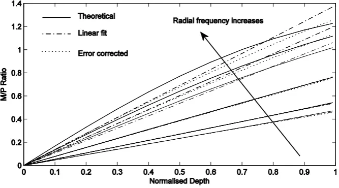
2.2. Model Verification

The designed model was verified by working backwards to determine how well the designed filters fitted the theoretical M/P ratio. To enable an accuracy comparison with Watanabe’s filters, the kernel size (7x7) and the number of frequency samples (32x32) were chosen as in [4]. As Watanabe [4] have not published a verification of their designs, and the numerical results for their 32 x 32 frequency responses were not available, direct comparison of the results was not feasible at this stage. Full comparisons can be made only on the estimated depth maps as described later. However a rough comparison with their filters was done by transforming their 7x7 spatial kernels into 32 x 32 frequency characteristics. These results have been presented in Section 3.

In the verification process, the frequency band up to which the M/P ratio remained monotonic was determined. In this section, the results have been based on the defocus condition:

pixels

Fe

e

307

.

2

=

, that was used by Watanabe [4] when they obtained their filters. Using the

equations in the Appendix, the following constants were calculated for the experiment:- e = 17.746 pixels, Fe = 7.6923, maximum blur diameter = 4.1614 pixels, focal length, f = 50mm, kernel size, ks

= 7 pixels, and aperture, d = 6.5mm. Again, by using the equations in the Appendix, the pattern frequency range used by the DfD calculation was 0.2857 ≤ fr ≤ 0.3164 pixels

-1

[image:9.612.136.470.400.585.2]

between the theoretical M/P ratio and both the linear and the error corrected models have been provided in Table 1. It can be inferred that the filters devised by the new method fit well with the theoretical ones. More results for both simulated and real images have been presented in later sections.

Table 1. Comparison of MSE between the Linear and Error Corrected Models

Figure 3. Model verification

3. Comparison with the Previous Filters

This section provides a comparison between the filters designed by the Two Step Polynomial approach presented in Section 2 with those designed by Watanabe [4]. The 7x7 filter coefficients of

Radial frequency

(pixels-1)

MSE between M/P

ratio and Linear Model

MSE between M/P ratio and Error Corrected Model

0.3141 0.0703 0.0636

0.3125 0.0630 0.0533

0.3078 0.0499 0.0397

both models were transformed into their equivalent 32x32 sample frequency responses, and verified as to how well they fit the theoretical M/P ratio. Figure (4a) shows the theoretical M/P ratio, Watanabe’s Model [4], and the Two Step Polynomial results. The maximum texture frequency

applicable for the defocus condition pixels Fe

e

307 . 2

= has been shown as it was the most curved.

Visually the proposed filters have provided a better fit. For a quantitative comparison figure (4b) shows the accumulated RMS errors for Watanabe’s [4], and the Two Step Polynomial filters for all the frequencies within the applicable range. The RMS error was significantly lower for the Two Step Polynomial method particularly for normalised depths approaching one.

Figure 4. (a) Normalised depth vs. Theoretical M/P ratio for both models, (b) RMSE between theoretical M/P ratio and filter models

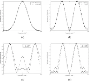
Next the normalised gain magnitude response of the filters was compared. Taking 1D slices through the 2D responses, as shown in Figure (5), filters Gm1 and Gp1 are similar for each model. However,

there is a considerable dissimilarity in the response of the correction filter Gp2. It is noted that Gp2

designed by the new model has a sharper transition between pass and stop bands, and a higher DC magnitude compared to Watanabe and Nayar’s. This DC does not propagate in the depth estimation since the pre-filter suppresses any frequency response below the minimum cut-off frequency. Moreover the pre-filter designed by the new method has a smooth roll-off in the transition band compared to a sharp transition for Watanabe’s. A sharp transition can propagate a ringing effect [23].

[image:10.612.134.481.221.390.2]

[image:11.612.164.453.169.430.2]

have been shown in Figure (6). The mean depth error and standard deviation for the Two Step Polynomial model was 0.0454 and 0.0128, and for Watanabe’s model 0.3615 and 0.2008 respectively. From Figure 6 and the standard deviation results it can be inferred that the depth map generated by the new filters is smoother and more planar than Watanabe’s. This is because Watanabe’s filters are not as circularly symmetric as the new set.

Figure 5. Magnitude responses of (a) Gm1, (b) Gp1, (c) Gp2 and (d) Pre-filter

[image:11.612.164.449.521.655.2]

4. Depth Estimation Experiments

This section describes the results from a series of experiments designed to measure the depth accuracy of the DfD calculation when the new filters are used, and to compare them with Watanabe’s published set [4]. The DfD algorithm described in [4] was coded and used to estimate the depth in each case. A full description of the algorithm can be found in [4]. For our particular implementation we smoothed the recovered depth map from each calculation using a 9x9 median filter as a post-process.

The experiments used both simulated and real images, each with 256 grey levels and a resolution of 400x400 pixels. They were selected to enable estimates of both the depth accuracy over a range of distances, and the dependence of the depth accuracy on the characteristics of the surface pattern of the object being measured. To enable a comparison the same input images were used in testing both the proposed filters and Watanabe’s. Section 4.1 concerns simulated images. Firstly single spatial frequency patterns were used to render the surface of a 3D staircase object and the depth accuracy estimated for each step. Then a more complex and spatially varying pattern was used to render each step. In Sections 4.2 and 4.3 tests on naturally occurring textures and a range of actual objects from flat planes to composite objects have been reported.

4.1. Experimental Results with Simulated Images

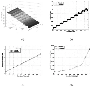
Figure 7. (a) Actual vs. Estimated depth at various normalised depths using the proposed and Watanabe’s filters, (b) Standard deviation at these depths for both filter models

To verify the invariance of the filter coefficients to the image texture, a pattern set devised by Watanabe [4] that contained several differently texture stripes was used. Seven stripes had patterns with narrow spectral densities (PSD) centered on differing frequencies, and the remaining three had wide PSD patterns. The original pattern set was defocused using the pillbox psf to simulate a 3D staircase structure.

Figure 8. (a) 3D view of the estimated depth, (b) 1D plot of the estimated depth, (c) Actual vs. estimated depth for filters designed by both the models, (d) Standard deviation at different depths

[image:13.612.146.469.69.221.2] [image:13.612.154.462.374.668.2]

Figure (8a) shows the estimated depth in 3D of the staircase using the new filters, and Figure (8b) shows a randomly section through the staircase for the filters designed by the new method and for those designed by Watanabe’s. The linearity of the depth estimates for both the filter sets has been compared in Figures (8c) and (8d). It can be inferred that the filters designed by the new method are invariant to texture and provide a slightly better fit to the actual depth than Watanabe’s. The relatively poor results from the higher steps are due to the use of the lower frequency section of the pattern there. In the following sections, experiments have been reported using real images and the accuracy of the depth estimated using both sets of filters has been compared.

4.2. Experiment with a random textured natural pattern: Abrasive Paper

This section provides depth estimation results using defocused images of a sheet of glass paper in a plane perpendicular to the optical axis. Eventually this pattern also served as the reference pattern used to calibrate the system since the PSD was wide within the working frequency range for the defocus condition. To enable a useful accuracy comparison with Watanabe [4], the defocus

condition was again set to pixels Fe

e

307 . 2

= . Using the equations in the Appendix, the working

range was calculated to be 56mm, this was quite short but was limited by the pixel size of the camera and the aperture used. A larger pixel size or a narrower aperture would have provided an increase in the range [17].

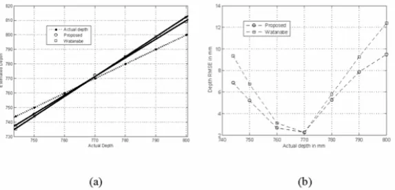
Figure 9. (a) Actual vs. Estimated distance (mm), (b) RMSE vs. Actual distance (mm)

[image:14.612.163.450.382.520.2]

accuracy over Watanabe’s for these natural textures. The next section provides depth results for actual 3D objects with natural textures.

4.3. Experiments with 3D objects and Natural textures

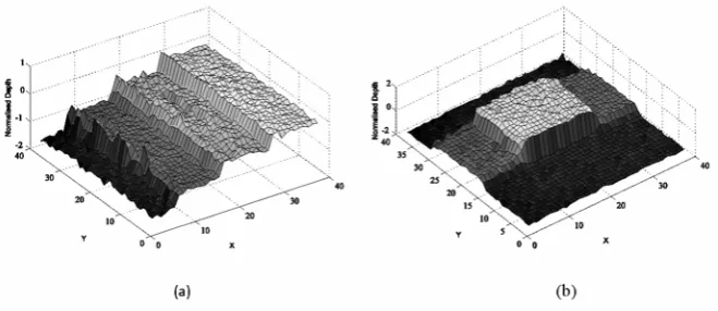
To complete the evaluation of the new set of filters, two real 3D objects with natural textures were measured. The objects were a multi-step staircase structures made from 3 pieces of mild steel on a background and a “T” structure made from natural wood. Figure (10) shows an original image of each structure, and Figure (11) the estimated depth maps. The shapes of the staircase and “T” can be identified easily in the depth maps. However, there were gaps between the steps on the staircase that were in deep shadow and this has resulted in large errors along the edges of each step. The objects and background were illuminated by a large area light source that has resulted in some specular reflections from their surfaces and hence less smooth depth maps than those obtained for the abrasive paper. As with human and stereo vision, that also require texture patterns for depth recovery, the shadows and specular reflections have resulted in some problems for DfD. Image noise introduced in the sensors or by the camera electronics has been identified as a source of errors for some image processes [24], but for DfD such noise is rejected by the algorithm as there is no correlation between the noise in each of the differently defocused images captured. To prove this noise was reduced in each input image by averaging several images for each defocus condition. The noise in the depth map was found to be independent of image noise.

[image:15.612.142.472.543.686.2]

Figure 10. Near-focused images of (a) Staircase, and (b) “T”

5. Conclusion

The proposed design procedure based on the Two step polynomial model was simple to perform, and provided a better fit to the theoretical M/P ratios than Watanabe’s filters [4] (Sections 2 and 3). Tests with simulated textures described in Section 3 proved that the two step polynomial filters were texture invariant and that they were more circularly symmetric than Watanabe’s. The tests described in Section 4 showed that the filters designed by the new model provided a better fit to the actual depth than those of the previous design. Generally, tests with real images of arbitrary natural textures (glass paper) resulted in slightly higher errors than for simulated images (Section 4.2) as the actual lens psf was defocusing the images as opposed to the theoretical cylindrical shaped psf that was used to model the M/P ratios. For the filters designed by the Two Step Polynomial approach the RMS error with respect to the distance was 0.9236% at the near-focused plane and 1.186% at far-focused, compared to 1.258% and 1.547% for Watanabe’s filters. From these results it can be inferred that the new filters estimated the depth at a higher accuracy than the previous filters.Moreover, the design procedure explained in Section 2 can be effectively applied for any defocus conditions by simply modelling the psf.

Appendix: Setting up and verifying the Working Distance for the

Rational Filters designed by the Two Step Polynomial Approach

Referring to Figure 1, given the defocus condition, D, and the far-focused object distance uf, the

working distance is uf - un, where un is the near-focused image distance. The f-number of the lens,

d f

F_e = . Where f is the focal length of the lens and d is the diameter of the aperture. The distance

between the near and far-focused images, 2e=2 *D Fe pixsize* * , where pixsize refers to the camera CCD element size which was 7.4μm for our camera and 13μm for Watanabe’s. The

far-focused image distance, _f f *

f

u f v

u f

=

− , and the near-focused distance vn= vf + 2e. Now

*

n n

n

v f u

v f

= −

.

In practice the working distance will be known and then the defocus condition can be calculated and

verified. Determine e =

2 *

n f

v

v

pixsize

−

pixels and

e

F e

D= pixels. Now D must satisfy the following

constraints:- (a) The maximum frequency that can be resolved, max fr=

*

0.73*

Fe pixsize

e

pixel

-1 ;

(b) The minimum frequency that can be resolved by the filter,

s r

k

f

2

size of the kernel (7 pixels); The factor of 0.73 comes from the maximum blur circle diameter,

s e

k F

e

73 . 0 2

≤ pixels and ensures a monotonic M/P ratio.

References

[1] P. Grossmann, Depth from focus, Pattern Recognition Letters, 5 (1) (1987) 63-69.

[2] Aamir Saeed Malik and Tae-Sun Choi, A novel algorithm for estimation of depth map using image focus for 3D shape recovery in the presence of noise, Pattern Recognition, 41 (7) (2008) 2200-2225.

[3] A.P. Pentland, A new sense for depth of field, IEEE Transactions on Pattern Analysis and Machine Intelligence, 9 (4) (1987) 523-531.

[4] M. Watanabe and S.K. Nayar, Rational filters for passive depth from defocus, International Journal of Computer Vision, 27 (3) (1998) 203-225.

[5] M. Subbarao and T.C Wei, Depth from defocus and rapid auto focussing: a practical approach, Proc. of IEEE Computer Society Conference on Computer Vision and Pattern Recognition, Champaign, Illinois, USA, 773-776, 1992.

[6] M. Subbarao and G. Surya, Depth from defocus: spatial domain approach, International Journal of Computer Vision, 13 (3) (1994) 271-294.

[7] J. Ens and P. Lawrence, Aninvestigation of methods for determining depth from defocus, IEEE Transactions on Pattern Analysis and Machine Intelligence, 15 (12) (1993) 97-108. [8] O. Ghita and P.F. Whelan, Real time 3D estimation using depth from defocus, Proc. of Irish

Machine Vision and Image Processing Conference, Dublin City University, Ireland, 167-181, 1999.

[9] A.N. Rajagopalan and S. Chaudhuri, An MRF model-based approach to simultaneous recovery of depth and restoration from defocused images, IEEE Transactions on Pattern Analysis and Machine Intelligence, 21 (7) (1999) 577-589.

[10] A.N. Rajagopalan and S. Chaudhuri, Depth from defocus: a real aperture imaging approach, Springer, New York, USA, 1999.

[11] P. Favaro and S. Soatto, A geometric approach to shape from defocus, IEEE Transactions on Pattern Analysis and Machine Intelligence, 27 (3) (2005) 406-417.

[12] P. Favaro and S. Soatto, Learning shape from defocus, Proc. of 7th European Conference of Computer Vision, Copenhagen, Denmark, Part 2, 735-745, 2002.

[13] F. Deschenes, D. Ziou, P. Fuchs, Improved estimation of defocus blur and spatial shifts in spatial domain: a homotopy-based approach, Pattern Recognition, 36 (9) (2003) 2105-2125. [14] F. Deschenes, D. Ziou, P. Fuchs, A homotopy-based approach for computing defocus blur

and affine transform simultaneously, Pattern Recognition, 41 (7) (2008) 2263-2282.

[15] D. M. Tsai and C. T. Lin, A moment preserving approach for depth from defocus, Pattern Recognition, 31 (5) (1998) 551-560.

[17] A.N. Joseph Raj, Accurate Depth from defocus estimation with video rate implementation, Ph.D. Dissertation, Univ. of Warwick, Coventry, U.K. Dec 2009.

[18] M. Watanabe and S.K. Nayar, Telecentric optics for focus analysis, IEEE Transactions on Pattern Analysis and Machine Intelligence, 19 (12) (1997) 1360-1365.

[19] A.N.J. Raj and R.C. Staunton, Estimation of image magnification using phase correlation, Proc. International Conference on Computational Intelligence and Multimedia Application, Sivakasi, India Vol. 3, 490-494, 2007.

[20] T.J. Schultz, Multiframe image restoration, in Handbook of Image and Video Processing, Al Bovik ed. Academic Press, San Diego, CA, USA, 175-189, 2000.

[21] C. D. Claxton and R. C. Staunton, Measurement of the point-spread function of a noisy imaging system, Journal of the Optical Society of America A, 25 (2008) 159-170.

[22] D. Marr and E. Hildreth, Theory of edge detection, Proc Royal Society London, B207 (1980) 187-217.

[23] Jae S. Lim, Two Dimensional Signal and Image Processing, Prentice Hall Inc, New Jersey, USA, 1990.