Original citation:
Sinclair, Lucas, Ijaz, Umer Z., Jensen, Lars Juhl, Coolen, Marco J.L., Gubry-Rangin, Cecile, Chroňáková, Alica, Oulas, Anastasis, Pavloudi, Christina, Schnetzer, Julia, Weimann, Aaron, Ijaz, Ali, Eiler, Alexander, Quince, Christopher and Pafilis, Evangelos. (2016) Seqenv : linking sequences to environments through text mining. PeerJ, 4 . e2690.
Permanent WRAP URL:
http://wrap.warwick.ac.uk/85051
Copyright and reuse:
The Warwick Research Archive Portal (WRAP) makes this work of researchers of the University of Warwick available open access under the following conditions.
This article is made available under the Creative Commons Attribution 4.0 International license (CC BY 4.0) and may be reused according to the conditions of the license. For more details see: http://creativecommons.org/licenses/by/4.0/
A note on versions:
The version presented in WRAP is the published version, or, version of record, and may be cited as it appears here.
Submitted26 July 2016
Accepted 14 October 2016
Published20 December 2016
Corresponding authors
Christopher Quince, [email protected],
[email protected] Evangelos Pafilis, [email protected]
Academic editor
Timothy Read
Additional Information and Declarations can be found on page 14
DOI10.7717/peerj.2690
Copyright
2016 Sinclair et al.
Distributed under
Creative Commons CC-BY 4.0
OPEN ACCESS
Seqenv
: linking sequences to
environments through text mining
Lucas Sinclair1,*, Umer Z. Ijaz2,*, Lars Juhl Jensen3
, Marco J.L. Coolen4 , Cecile Gubry-Rangin5
, Alica Chroňáková6
, Anastasis Oulas7,8 , Christina Pavloudi8
, Julia Schnetzer9
, Aaron Weimann10
, Ali Ijaz11 , Alexander Eiler1
, Christopher Quince12
and Evangelos Pafilis8
1Department of Ecology and Genetics, Limnology, Uppsala University, Uppsala, Sweden
2Infrastructure and Environment Research Division, School of Engineering, University of Glasgow, Glasgow,
United Kingdom
3The Novo Nordisk Foundation Center for Protein Research, Faculty of Health and Medical Sciences,
University of Copenhagen, Copenhagen, Denmark
4Western Australia Organic and Isotope Geochemistry Centre (WA-OIGC), Department of Chemistry, Curtin
University of Technology, Bentley, WA, Australia
5Institute of Biological & Environmental Sciences, University of Aberdeen, Aberdeen, United Kingdom 6Institute of Soil Biology, Biology Centre, Czech Academy of Sciences, České Budějovice, Czech Republic 7Bioinformatics Group, The Cyprus Institute of Neurology and Genetics, Nicosia, Cyprus
8Institute of Marine Biology Biotechnology and Aquaculture (IMBBC), Hellenic Centre for Marine Research
(HCMR), Heraklion Crete, Greece
9Department of Molecular Ecology, Microbial Genomics and Bioinformatics Group, Max Planck Institute for
Marine Microbiology, Bremen, Germany
10Computational Biology of Infection Research, Helmholtz Centre for Infection Research, Braunschweig,
Germany
11Hawkesbury Institute for the Environment, University of Western Sydney, Hawkesbury, Sydney, Australia 12Warwick Medical School, University of Warwick, Warwick, United Kingdom
*These authors contributed equally to this work.
ABSTRACT
Understanding the distribution of taxa and associated traits across different envi-ronments is one of the central questions in microbial ecology. High-throughput sequencing (HTS) studies are presently generating huge volumes of data to address this biogeographical topic. However, these studies are often focused on specific environment types or processes leading to the production of individual, unconnected datasets. The large amounts of legacy sequence data with associated metadata that exist can be harnessed to better place the genetic information found in these surveys into a wider environmental context. Here we introduce a software program,seqenv, to carry out precisely such a task. It automatically performs similarity searches of short sequences against the ‘‘nt’’ nucleotide database provided by NCBI and, out of every hit, extracts–if it is available–the textual metadata field. After collecting all the isolation sources from all the search results, we run a text mining algorithm to identify and parse words that are associated with the Environmental Ontology (EnvO) controlled vocabulary. This, in turn, enables us to determine both in which environments individual sequences or taxa have previously been observed and, by weighted summation of those results, to summarize complete samples. We present two demonstrative applications ofseqenv
and its utility in the fields of environmental source tracking, paleontology, and studies of microbial biogeography. To installseqenv, go to:https://github.com/xapple/seqenv.
SubjectsBioinformatics, Ecology, Environmental Sciences, Microbiology
Keywords Bioinformatics, Ecology, Microbiology, Genomics, Sequence analysis, Text processing, Statistics, Pipeline, Open source software
INTRODUCTION
The annotation of DNA sequences, i.e., attaching meaningful labels to them, is key to the interpretation of genomics data. In essence, this process gives context to a sequence. For instance, annotation reveals the taxon from which the sequence was derived (Wang et al., 2007) and/or the gene families and potential functions (Juncker et al., 2009). However, one type of annotation for which no automated bioinformatics pipeline currently exists is the annotation to the environmental source. In other words, determining the types of environ-ment in which a given sequence has previously been found. We introduce a new program titled ‘‘seqenv’’ which addresses this gap, automatically labeling sequences to the Envi-ronmental Ontology (EnvO) (Buttigieg et al., 2013). We apply this bioinformatics pipeline to two datasets of environmental marker genes derived from terrestrial archaeal ammonia oxidizers (AOA) (Gubry-Rangin et al., 2011) and the Black Sea plankton paleome (Coolen
et al., 2013). This method reveals hitherto unknown patterns in AOA diversity, and adds
to our understanding of the geological history of the Black Sea.
Annotating sequences to environments has become increasingly relevant as a result of the growing application of environmental genomics to microbiology. In environmental ge-nomics, microbial DNA is extracted directly from an environment and then sequenced, pos-sibly following PCR amplification of target marker genes such as the 16S rRNA gene (Logares
et al., 2012). The result is a catalog of the microorganisms present in a particular sample.
One of the first interrogations concerning such samples is to know what other environments these organisms have been found in. The answer can reveal ecologically relevant insight about those organisms and may provide evidence for contamination from other environ-ments. There exists a wealth of information in available databases (most notably the ones provided by NCBI) which can be used to gain a detailed overview of the biogeography of particular sequence varieties. The strategy adopted inseqenvis to take input sequences and match them against the NCBI’s database using the time-tested BLAST search algorithm
(Altschul et al., 1990).
Environmental Ontology (http://environmentontology.org/) (or EnvO) provides an ontol-ogy for this concise, controlled vocabulary for the description of environments. EnvO also has the appeal of having been adopted by the Genomics Standards Consortium for metadata associated with environmental sequence submission (Field et al., 2014). The terms found as-sociated with each sequence are then collated together to provide its environmental context. This environmental annotation scheme can be applied to any type of sequence, protein coding or ribosomal RNA. The sequences can be derived from a particular taxonomic grouping but they can also correspond to operational taxonomic units (OTUs) used as prox-ies for taxa in environmental sequencing studprox-ies (Blaxter et al., 2005). In either case, the na-ture and diversity of environments associated with a particular microorganism can elucidate and bring light to its ecology. Additionally, if OTUs are used,seqenvcan also incorporate their abundances across samples. This furnishes a sample-level description of the EnvO terms produced by simply summing the terms associated with each OTU weighted by their relative abundance in the sample. These tables can then be used as a basis for multivariate statistics that contrast communities in terms of the environmental terms associated with their constituent organisms. This novel approach is a powerful means for exploring sample level differences in the origin of community constituents.
Recently, a method has been developed for automatically associating geographic longitude and latitude coordinates to Genbank records through rule based text mining of as-sociated PubMed Central articles (Tahsin et al., 2016). Our approach is distinguished from this in two ways. Firstly, we start from sequences rather than records, allowing us to examine the distribution of environmental contexts within a certain level of sequence similarity. Secondly, we associate to EnvO terms rather than to geographic coordinates. This makes
seqenvmore relevant to exploring the ecology of microbes, determining the distribution of OTUs across environment types, as opposed to tracking viral outbreaks which was a previous focus (Tahsin et al., 2016). The information thatseqenvautomatically generates can answer similar questions to those addressed previously (Chaffron et al., 2010), where co-occurrence of OTUs across sampling sites was examined and isolation sources were classified to EnvO terms through text matching. We provide this functionality in a single coherent software pipeline and promote user-friendliness.
ATCGCGTCAGTCATGCAT GCATCGTAATCGTCGCGT CAGTCATGCATGCATCGT AATCGATCGCGTCAGTCA TGCATGCATCGTAATCGA TCGCGTCAGTCATGCATG CATCGTAATCG OTU_1 also called C1
User input
Note: There is only one sequence in this example here. It is also called an "OTU".
The whole process is repeated the same way for every
sequence
independently. 343206452
G-id (global identifier) Search result against NT
database.
(maximum 10 hits are found so maximum 10 G-ids are
retrieved)
324498760 G-id (global identifier)
324498739G-id (global identifier)
Every GI has 0 or 1 isolation source.
(can be the same as another GI)
the deepest lake mud of the lake Mariana Trench
Isolation source
marine water of Arraial do Cabo wetland system Isolation source None marine biome ENVO:00000447 ENVO term lake ENVO:00000020 ENVO term marine habitat ENVO:00000569 ENVO term wetland ENVO:00000043 ENVO term 324499999
G-id (global identifier)
324498738
G-id (global identifier)
My bath
Isolation source None
Count it 1.0
Count it 1.0
Count it 1.0 "seq_to_gis"
All numbers are fake This figure describes a plan for processing data, not results.
Tue Sep 20 2016 Last modified:
Description of seqenv internal pipeline structure
Lucas Sinclair, [email protected]
lake ENVO:00000020
ENVO term
This OTU is 25% lakish This OTU is 25% marine biomish This OTU is 25% marine habitish This OTU is 25% wetlandish
Result
This GI is 200% lake
Result for 343206452
These are the "flat" results per GI.
(without special normalization rules such
as backtracking)
This GI is 100% marine biome This GI is 100% marine habitat This GI is 100% wetland
Result for 324498760
Every isolation source has 0, 1 or more ENVO terms
attached to it.
(NB: can be duplicates)
Count it 1.0
Count it 1.0
Counts per ENVO term.
This GI is 100% marine biome This GI is 100% marine habitat This GI is 100% wetland
Result for 324499999
None
Result for 324498738
None
Result for 324498739 Don't count it
Don't count it 34250972312
Pubmed ID
523452344523
Pubmed ID
213421343343Pubmed ID
Note: G-ids with no isolation source associated are not considered in seqenv
Note: G-ids with no recognized envos in their isolation source text are not considered
in seqenv
[image:5.612.40.572.79.375.2]Note: The "--proportional" option is active.
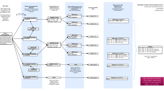
Figure 1 Schematic of the internal functioning of theseqenvpipeline.This figure details how EnvO term frequencies are computed. The num-bers provided are fictional as the schematic focuses on representing the internal functioning of the pipeline and does not illustrate a concrete case. As each inputted short DNA sequence is processed independently in all but the last stages ofseqenv, only one input sequence is shown here.
MATERIALS AND METHODS
Theseqenvpipeline proceeds through the following steps, as illustrated diagrammatically inFig. 1. The input is a user-supplied FASTA file containing thousands of DNA sequences and, optionally, a frequency file containing the frequency counts of the sequences across multiple samples. This file takes the form of a tab delimited text file containing the count matrix. In typical usage, the sequences would correspond to the consensus sequences of OTUs and the matrix would represent their frequencies across samples. After the following procedure, multiple outputs are generated:
1. The first step thatseqenv executes is the parsing of the FASTA input file. All the sequence names are removed and replaced by a place-holder title following the sequence ‘‘C1’’, ‘‘C2’’, ‘‘C3’’, etc. In this fashion, problems caused by odd encodings or ambiguous characters are circumvented.
3. Next, every remaining sequence is compared to a database of the user’s choice. By default, the ‘‘nt’’ (nucleotide) database provided by NCBI is used and the BLAST algo-rithm is chosen to carry out the similarity search (Altschul et al., 1990). This step is the most costly computationally. It can, however, be parallelized byseqenvon multi-core systems by performing a simple and automatic input-chopping strategy.
4. Taking all the results from the sequence similarity search, the best hits are selected by filtering them according to thee-value of the comparison, the coverage of one sequence against the other, the identity between one sequence and the other, and a maximum number of targets for each input sequence. These parameters default to 0.0001, 0.97, 0.97, and 10 respectively.
5. For every search hit from every input sequence, the corresponding GenInfo Identifier (GI) of the homologous target within the database is recorded. This creates a table that links every input sequence to zero, one or more GI numbers.
6. Then, we collect the ‘‘isolation source’’ text entries associated to all of the GI numbers recorded in the previous step, provided the GI number was associated with such a field in NCBI’s database, failing which it is discarded. No internet connection is required as all text entries are stored in an SQLite3 database and can be accessed locally byseqenv. This database links every GI number to its PubMed identifier, along with its isolation source text.
7. Using all the isolation source texts collected in the previous step and a text mining module, we proceed to identify all terms that contain some type of environmental information. Words such ‘‘glacier’’, ‘‘pelagic’’ or ‘‘forest’’ are extracted and connected to the controlled EnvO vocabulary. This consists of a hierarchically organized network of descriptive terms. In particular, the frequency of occurrence of each word is noted. Concretely, this is done offline by using a named entity recognition (NER) system. The NER algorithm is an optimized dictionary-based tagger, it searches for keywords associated with each ENVO term but also using a stop-list of problematic words (Pafilis
et al., 2015). The ability of the NER engine to tag text with ENVO terms was evaluated
inPafilis et al. (2015)through comparison to a manually curated corpus this resulted in
87.8% precision and 77.0% recall, corresponding to an F1 score of 82.0%. The results were placed into an SQLite3 database that is automatically downloaded on the first run ofseqenv.
to the same study. In all cases, the rows of the matrix are normalized to 1.0, such thatsj,k =s0j,k/Pls0j,l, where we are denoting the raw counts by s0j,k. The default normalization strategy is ‘‘flat’’.
9. If the user supplied a frequency matrix (c.f. second step), we are able to describe every one of the original biological samples by a set of EnvO terms and frequencies that are simply the sum of the term vectors over all sequences, weighted by the abundance of that sequence in the sample. Equivalently, the sample term matrixNelementsni,k, is the matrix product of the frequency matrixFelementsfi,j and the sequence-term matrix, i.e.,n0i,k=P
jfi,jsj,k. Normalizing by the total frequency in the sample, such thatni,k=n0i,k/
P
ln
0
i,l, we obtain sample term vectors such as, translated to English: ‘‘Sample Z is 25% brackish estuary, 25% river and 50% wetland’’.
10. Other options are available to the user to further modify and filter the results. The ‘‘backtracking’’ option, when activated, will propagate frequency counts up the acyclic directed graph described by the ontology for every EnvO term identified by the text mining module. The ‘‘restrict’’ option, when specified by passing a given EnvO identifier (e.g., ENVO:00010483), will force the output to contain only descendants from a single EnvO term. In effect, all other terms that are not reachable through the given node in the ontology graph are removed.
11. The first output that is produced is a table serialized in the format of a tab-delimited plain text file (TSV) representing the composition of each input sequence according to the EnvO terms associated to them, i.e., the matrixS. The columns represent input sequence and rows represent the normalized weight of EnvO terms.
12. If the user provided a frequency matrix (as described in step 2), the program can produce a similar TSV table representing the composition of each biological sample according to the EnvO terms associated to them, i.e., the matrix N. In this case, columns represent samples and rows represent EnvO terms. Each value corresponds to the normalized weight of the EnvO term in the corresponding sample.
13. For each sample, a visual representation of the hierarchy of the EnvO terms occurring in the isolation source of its imputed close relatives can be made. A PDF file is generated for each sequence and, if the user provided an abundance table, for each sample. In addition, every PDF has a corresponding DOT file which can be viewed and manipulated with the Graphviz software.
14. Other intermediary outputs are available as well, such as the output of the similarity search and a precise list of every EnvO term found in each input sequence.
Theseqenvpackage is written in Python. The code follows a clean architecture, is commented and object-oriented. It is free and open-source carrying an MIT license. It is available on github here:https://github.com/xapple/seqenv. It can be installed on any computer with Python by simply typing: ‘‘pip install seqenv’’ in your shell.
RESULTS
sources and the air (Comte et al., 2014), as well as a survey of bacterial diversity along a 2,600 km river continuum (Savio et al., 2015), and a study of hydrogenase genes in lake sediments (Couto et al., 2015).
Here, to further illustrate its utility, we will apply it to two published datasets and demonstrate that it provides additional insights into the processes that structure microbial communities not evident in the original analyses. These two examples comprise:
1. A survey of archaealamoAgene data from 45 British soils, originating from a broad range of pH (min. 3.5, max. 8.7, median 6.2) (Gubry-Rangin et al., 2011). The sequences were generated by bidirectional 454 pyrosequencing of part of theamoAgene, reads were denoised with AmpliconNoise (Quince et al., 2011), overlapped and further error checked by removing those with stop codons when translated into amino acids. For this part of the analysis, we generated operational taxonomic units (OTUs) at 5% sequence divergence using average linkage hierarchical clustering. This will be higher resolution than species (Pester et al., 2011), corresponding to ecotypes with well defined environmental preferences. This procedure resulted in just 67 OTU sequences. All sequences were from archaeal ammonia oxidizers (AOAs) as described previously
(Gubry-Rangin et al., 2011).
2. The Black Sea Paleome. This study included 454 pyrosequencing of 18S rRNA gene amplicons from 48 deep sediment samples collected from the Black Sea enabling the reconstruction of microbial eukaryote populations up to 11,400 years in the past. The V1–V3 region was sequenced as described previously (Coolen et al., 2013). Reads were denoised with AmpliconNoise and OTUs constructed at 3% sequence divergence using average linkage hierarchical clustering as species proxies (Quince et al., 2011). A total of 1,748 OTUs were obtained.
Patterns of ammonia oxidizing archaea (AOA) habitat usage
In total 67 OTUs were observed across the 45 samples. These OTUs have been previously demonstrated as having well defined pH preferences (Gubry-Rangin et al., 2011). For each OTU, we calculated the mean of its pH range as the weighted averaged of the samples it was observed in, i.e.,:
¯ Ys=
N
X
n=1 xn,sYn,
whereY¯sis the mean pH range for OTUsandxn,sis the relative abundance ofsin sample
NB: darker nodes weigh more Is Part Located a of in terrestrial habitat habitat environmental material soil bulk soil
NB: darker nodes weigh more Is Part Located a of in sludge anthropogenic environmental material environmental material environmental feature biome
mouth watercourse water body
hydrographic feature spring
soil terrestrialhabitat habitat marine water body compost agricultural environmental material aquatic biome physiographic
feature geographicfeature
tidal mudflat saline marsh coastal wetland mudflat saline wetland saline hydrographic feature marsh wetland coast lake stream river volcano volcanic feature water grassland soil grassland volcanic hydrographic feature waste stream mouth river mouth estuary marine biome lake sediment sediment sea marine feature hot spring hydrothermal vent waste water freshwater wetland
A
OTU #46
pH 3.5
OTU #66
pH 8.5
B
NB: darker nodes weigh more
[image:9.612.186.576.88.418.2]Is Part Located a of in terrestrial habitat habitat environmental material soil bulk soil
Figure 2 The EnvO terms associated with two AOA OTUs.For each original inputted sequence,seqenv outputs a network representing the EnvO terms identified. Two examples of such hierarchical ontologies are shown. The two OTUs chosen had a mean pH of 3.5 and 8.5. The intensity of the node’s background color reflects the frequency of that term within hits. Gray indicates the lowest frequency recorded and darker shades of yellow to orange indicate higher frequencies.
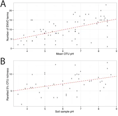
two and fifteen EnvO terms associated with them in total respectively. In all, we obtained EnvO terms for 66 OTUs. The 67th OTU did not match to any sequences carrying environmental information in the database. InFig. 3A, the total number of terms found for each OTU as a function of its preferred pH range is plotted. A significant positive correlation between the diversity of habitats and the pH of the samples the organism was found (adjustedR-squared: 0.274,p-value: 3.85e−06). Another weaker but still significant
positive association is observed between sample pH and total OTU diversity (adjusted
R-squared: 0.131,p-value: 0.00922).
0 5 10 15 20
4 5 6 7 8 9
Mean OTU pH
Number of EN
VO terms
5 10
4 5 6 7 8 9
Soil sample pH
Rarefied 5%
O
TU ri
chness
A
[image:10.612.184.580.87.478.2]B
Figure 3 EnvO terms and OTU richness against mean OTU pH.(A) shows the total number of EnvO terms against OTU pH. The dashed red line indicates a linear regression of number of EnvO terms with OTU pH (adjustedR-squared: 0.2742,p-value: 3.85e−06). (B) shows the community OTU diversity against sample pH for the AOA dataset. OTU richness was calculated after rarefying to 1,000 reads. Linear regression of sample diversity against pH (adjustedR-squared: 0.1305,p-value: 0.009217).
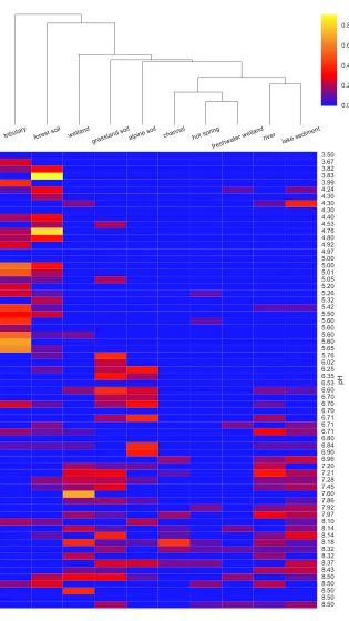
is possible using the left out samples. Additionally, estimates of variable importance can be obtained by comparing accuracy of prediction with and without randomly permuting the variable of interest. This is measured by the statistic: percentage mean decrease of accuracy (%IncMSE). We fitted a Random Forest using therandomForestR package (R Core Team,
2014;Liaw & Wiener, 2002). The model explained 34.6% of the variation in pH preference.
InFig. 4, we visualize the weights of the top ten most important terms as determined by %IncMSE across OTUs ordered by their pH preference.
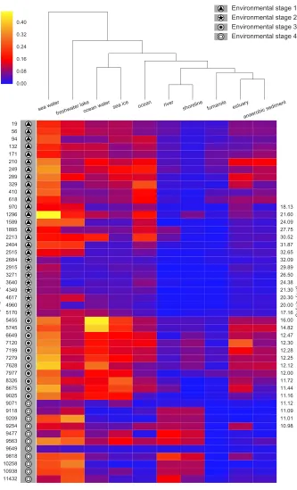
Environmental stages of the Black Sea paleome
−1.0 −0.5 0.0 0.5 1.0 − 1.0 − 0.5 0.0 0.5 NMDS1 NMDS2 ● ● ● ● ● ● ● ● ● ● ● ● ● ● ● ● ● ● ● ● ● ● ● ● ● ● ● ● ● ● ● ● ● ● ● ● ● ● ● ● ● ● ● ● ● ● ● ● ● ● ● ● ● ● ● ● ● ● ● ● ● ● ● ● ● ● ● ● ● ● ● ● ● ● ● ● ● ● ● ● ● ● ● ● ● ● ● ● ● ● ● ● ● ● ● ● 9071 9649 9025 19 171 329 11432 2515 2684 5170 5455 ● ● ● ● ● ● ● ● ● ● ●
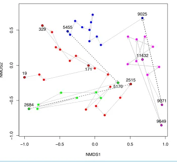
Figure 5 NMDS plot of Black Sea plankton 18S rRNA samples.Non-metric multidimensional scaling (NMDS) of OTU relative abundances with Bray–Curtis distances were used to ordinate the 18S rRNA Black Sea plankton samples in two dimensions. The age of key samples are indicated together with the En-vironmental Stage: ES4 (magenta), ES3 (blue), ES2 (green) and ES1 (red). Arrows indicate the temporal succession of samples, and dotted arrows represent the transition between environmental stages.
Stages’’ (ES) in the geological evolution of the Black Sea that apply to this depth series on the basis of fossil evidence and isotope ratios:
• ES4: Lacustrine interval (∼11.4–9.0 kyBP). During this lacustrine phase the Black Sea
was disconnected from the Mediterranean Sea due to low sea levels. This phase ends with the initial marine inflow (IMI) as rising sea levels, due to the end of the ice age 11,700 years ago, resulted in the connection of the Black Sea to the Mediterranean.
• ES3: A period of increasing salinity (∼9.0–5.2 kyBP) corresponding to the warm and
moist mid-Holocene climatic optimum.
• ES2: Establishment of modern environmental conditions (∼5.2–2.5 kyBP) and further
increasing salinity associated with the onset of the dry Subboreal.
• ES1: Freshening (∼2.5 kyBP to present) with onset of the cool and wet Subatlantic
climate and recent anthropogenic perturbations.
constructed differently, but we include it here for the sake of completeness. The trajectory through time of the samples together with their Environmental Stages are shown. From this it is clear that there is a coherent change in structure during the geological history of the Black Sea and that the samples cluster according to ES.
We next ranseqenvon the 1,748 18S rRNA OTU centroid sequences taking into account up to 100 matches with 97% overlap and 97% identity to the query. As above, we restricted the analysis to those terms that inherit from the term ENVO:00010483 ‘‘environmental ma-terial’’ and used the ‘‘flat’’ normalization option. The normalized term vectors for each OTU were then combined with the relative OTU frequencies across the 48 sediment samples to obtain the weighted frequency of terms across samples, as described above. In total we observed 99 separate EnvO terms across the 48 samples. As above, we used a random forest classifier to predict these environmental stages from the EnvO terms associated with each sample. This classifier had an error rate of 12.5%. InFig. 6we show the relative frequency of the ten most important terms in this classifier across the samples, ordered by age and with the ES groups indicated.
DISCUSSION
The two analyses presented above demonstrate the value of usingseqenvto associate EnvO terms with both individual OTUs and whole samples. In the analysis of AOA OTUs, we demonstrated a significant association between the pH that an OTU is adapted to and the diversity of environments that it is found. These results indicate that, as their optimum pH increases, the AOA OTUs are present across a greater diversity of habitats. As in the original study, a statistically significant relationship between sample OTU richness and pH was ob-served. That is, as the pH of a sample increases, more species are obob-served. We propose that these two observations may be connected: the fact that more environments appear accessible to the OTUs as the pH increases may generate the diversification of species that is reflected in the increasing sample richness with pH. At higher pHs, we might expect both of these relationships to be reversed due to increased competition with bacterial ammonia oxidizers.
In the geological history of the Black Sea, one of the key questions is the nature of that environment prior to the initial Mediterranean sea influx (IMI). For example, was it a Brackish environment, or was it akin to a freshwater lake landscape? In our Black Sea dataset analysis, we can note a discrete change in the EnvO terms associated with the samples at this event when we transition from ES4 to ES3. Prior to this point, terms such as ‘‘freshwater lake’’ and ‘‘river’’ are frequent, afterwards the samples are dominated by organisms associated with ‘‘sea water’’, ‘‘ocean water’’ and ‘‘estuary’’. The microbial community prior to the IMI comprised organisms associated with freshwater habitats, important evidence that the IMI was associated with a substantial increase in salinity.
CONCLUSION
analyzing and adding context to DNA sequence data. There may be areas in which our methodology could be improved for example by weighting terms in OTUs or samples using more sophisticated approaches from information retrieval. In any case, we believe that, in the future, seqenvwill contribute crucial insights and advances to the field of environmental metagenomics.
Abbreviations
16S 16 Svedberg sedimentation mark (non-SI unit)
ANOVA Analysis of variance
AOA Ammonia oxidising archaea
BLAST Basic local alignment search tool
BP Base pair (of nucleotides)
EnvO Environmental ontology
GI GenInfo identifier
HTS High-throughput (genetic) sequencing
MSE Mean squared error
NCBI National center for biotechnology information (in the US)
NER Named entity recognition
NMDS Non-parametric multidimensional scaling (ordination plot)
OTU Operational Taxonomic Unit
PCR Polymerase chain reaction
rRNA Ribosomal ribonucleic acid
TSV Tab separated values
ACKNOWLEDGEMENTS
Seqenvwas originally conceived in a series of<hackathons>supported by the European Union’s Earth System Science and Environmental Management COST Action. This project was titled ‘‘Microbial ecology & the earth system: collaborating for insight and success with the new generation of sequencing tools’’ and can be viewed at
http://www.cost.eu/domains_actions/essem/Actions/ES1103. We would like to thank the LifeWatchGreece project (http://www.lifewatchgreece.eu/) for their generous support in the organization of these meetings.
ADDITIONAL INFORMATION AND DECLARATIONS
Funding
fellowship (MR/M50161X/1). Cecile Gubry was funded by the Environment Research Council Fellowship (NE/J019151/1). The funders had no role in study design, data collection and analysis, decision to publish, or preparation of the manuscript.
Grant Disclosures
The following grant information was disclosed by the authors: Swedish Foundation for strategic research: ICA10-0015. NERC IRF: NE/L011956/1.
Novo Nordisk Foundation: NNF14CC0001.
European Commission FP7-REGPOT project MARBIGEN: #264089. LifeWatchGreece Research Infrastructure: 384676-94/GSRT/NSRF C&E. CLIMB project (MR/L015080/1): MR/M50161X/1.
Environment Research Council Fellowship: NE/J019151/1.
Competing Interests
The authors declare there are no competing interests.
Author Contributions
• Lucas Sinclair analyzed the data, wrote the paper, prepared figures and/or tables, reviewed
drafts of the paper, wrote the software productseqenvin Python in its entirety.
• Umer Z. Ijaz analyzed the data, wrote the bash-based original version ofseqenvuntil
version 0.8.0, after which, LS restarted the implementation. Tested the software.
• Lars Juhl Jensen contributed reagents/materials/analysis tools, reviewed drafts of the
paper, developed the NER software thatseqenvrelies on, as well as helped with using and installing it.
• Marco J.L. Coolen conceived and designed the experiments, reviewed drafts of the paper,
supplied the Black Sea dataset.
• Cecile Gubry-Rangin conceived and designed the experiments, reviewed drafts of the
paper, provided AOA data and expertise.
• Alica Chroňáková and Julia Schnetzer reviewed drafts of the paper, participated in the
first hackathon.
• Anastasis Oulas reviewed drafts of the paper, helped test the software.
• Christina Pavloudi reviewed drafts of the paper, participated in the hackathons, helped
test the software.
• Aaron Weimann reviewed drafts of the paper, participated in the second hackathon.
• Ali Ijaz participated in the second hackathon.
• Alexander Eiler reviewed drafts of the paper.
• Christopher Quince analyzed the data, wrote the paper, prepared figures and/or tables,
reviewed drafts of the paper.
• Evangelos Pafilis analyzed the data, reviewed drafts of the paper.
DNA Deposition
Data Availability
The following information was supplied regarding data availability:
https://github.com/xapple/seqenv.
REFERENCES
Altschul SF, Gish W, Miller W, Myers EW, Lipman DJ. 1990.Basic local alignment search tool.Journal of Molecular Biology215(3):403–410
DOI 10.1016/S0022-2836(05)80360-2.
Blaxter M, Mann J, Chapman T, Thomas F, Whitton C, Floyd R, Abebe E. 2005.
Defining operational taxonomic units using DNA barcode data. Philosophi-cal Transactions of the Royal Society of London. Series B360(1462):1935–1943
DOI 10.1098/rstb.2005.1725.
Breiman L. 2001.Random forests.Machine Learning 45(1):5–32
DOI 10.1023/A:1010933404324.
Buttigieg P, Morrison N, Smith B, Mungall CJ, Lewis SE, The ENVO Consortium. 2013.The environment ontology: contextualising biological and biomedical entities.
Journal of Biomedical Semantics4(1):43DOI 10.1186/2041-1480-4-43.
Chaffron S, Rehrauer H, Pernthaler J, Von Mering C. 2010.A global network of
coexisting microbes from environmental and whole-genome sequence data.Genome Research20(7):947–959DOI 10.1101/gr.104521.109.
Comte J, Lindström ES, Eiler A, Langenheder S. 2014.Can marine bacteria be recruited from freshwater sources and the air?The ISME Journal8(12):2423–2430
DOI 10.1038/ismej.2014.89.
Coolen MJL, Orsi WD, Balkema C, Quince C, Harris K, Sylva SP, Filipova-Marinova M, Giosan L. 2013.Evolution of the plankton paleome in the Black Sea from the Deglacial to Anthropocene.Proceedings of the National Academy of Sciences of the United States of America110(21):8609–8614DOI 10.1073/pnas.1219283110.
Couto JM, Ijaz UZ, Phoenix VR, Schirmer M, Sloan WT. 2015.Metagenomic se-quencing unravels gene fragments with phylogenetic signatures of O2-tolerant NiFe membrane-bound hydrogenases in lacustrine sediment.Current Microbiology 71(2):296–302DOI 10.1007/s00284-015-0846-2.
Field D, Sterk P, Kottmann R, De Smet JW, Amaral-Zettler L, Cochrane G, Cole JR, Davies N, Dawyndt P, Garrity GM, Gilbert JA, Glöckner FO, Hirschman L, Klenk H-P, Knight R, Kyrpides N, Meyer F, Karsch-Mizrachi I, Morrison N, Robbins R, San Gil I, Sansone S, Schriml L, Tatusova T, Ussery D, Yilmaz P, White O, Wooley J, Caporaso G. 2014.Genomic standards consortium projects.Standards in Genomic Sciences9(3):599–601DOI 10.4056/sigs.5559608.
Juncker AS, Jensen LJ, Pierleoni A, Bernsel A, Tress ML, Bork P, Von Heijne G, Valencia A, Ouzounis CA, Casadio R, Brunak S. 2009.Sequence-based feature prediction and annotation of proteins.Genome Biology10(2):206
DOI 10.1186/gb-2009-10-2-206.
Liaw A, Wiener M. 2002.Classification and regression by randomForest.R News 2(3):18–22.
Logares R, Haverkamp THA, Kumar S, Lanzén A, Nederbragt AJ, Quince C, Kauserud H. 2012.Environmental microbiology through the lens of high-throughput DNA sequencing: synopsis of current platforms and bioinformatics approaches.Journal of Microbiological Methods91(1):106–113 DOI 10.1016/j.mimet.2012.07.017.
Pafilis E, Frankild SP, Schnetzer J, Fanini L, Faulwetter S, Pavloudi C, Vasileiadou A, Leary P, Hammock J, Schulz K, Parr CS, Arvanitidis C, Jensen LJ. 2015.
ENVIRONMENTS and EOL: identification of environment ontology terms in text and the annotation of the encyclopedia of life.Bioinformatics31(11):45–1874
DOI 10.1093/bioinformatics/btv045.
Pester M, Rattei T, Flechl S, Gröngröft A, Richter A, Overmann J, Reinhold-Hurek B, Loy A, Wagner M. 2011.amoA-based consensus phylogeny of ammonia-oxidizing archaea and deep sequencing of amoA genes from soils of four different geographic regions.Environmental Microbiology14(2):525–539
DOI 10.1111/j.1462-2920.2011.02666.x.
Quince C, Lanzén A, Davenport RJ, Turnbaugh PJ. 2011.Removing noise from pyrose-quenced amplicons.BMC Bioinformatics12(1):38DOI 10.1186/1471-2105-12-38.
R Core Team. 2014.R: a language and environment for statistical computing. Vienna: Foundation for Statistical Computing.Available athttp:// www.R-project.org/.
Savio D, Sinclair L, Ijaz UZ, Parajka J, Reischer GH, Stadler P, Blaschke AP, Blöschl G, Mach RL, Kirschner AKT, Farnleitner AH, Eiler A. 2015.Bacterial diversity along a 2,600 km river continuum.Environmental Microbiology 17(12):4994–5007
DOI 10.1111/1462-2920.12886.
Tahsin T, Weissenbacher D, Rivera R, Beard R, Firago M, Wallstrom G, Scotch M, Gonzalez G. 2016.A high-precision rule-based extraction system for expanding geospatial metadata in GenBank records.Journal of the American Medical Informatics Association23(5):934–941DOI 10.1093/jamia/ocv172.