Counting People in Simultaneous Speech using Support
Vector Machines
Thomas Hogema
University of Twente P.O. Box 217, 7500AE EnschedeThe Netherlands
[email protected]
ABSTRACT
The purpose of this paper is to look at the feasibility of counting the number of simultaneous speakers from an au-dio clip. Currently, there are multiple ways to automat-ically count people. WiFi, Bluetooth, and video track-ing are some of the most common options. Each of these techniques has some downsides with regards to accuracy, usability or practicality. As an alternative, sound might be used to determine the number of people in a room. It could be used as an addition or alternative solution for presence detection. This paper will focus on counting the number of simultaneous speakers in an audio clip. In or-der to do this, we built a framework that can generate scenarios with overlapping speech and evaluate different features. The framework uses a support vector machine (SVM) for the prediction. First, the framework generated scenarios with overlapping speech. From these scenarios, features were extracted which are used to train the SVM. The primary feature we used was the Mel-frequency cep-stral coefficients (MFCC). Results show that, on average, we are able to estimate the number of speakers up to 17 people with a mean error close to zero.
Keywords
Speaker identification, machine learning, counting people, sound, sound features, presence detection, mfcc, svm
1.
INTRODUCTION
Today, presence detection is used for a variety of appli-cations. In office environments, it can be used to auto-matically control the indoor climate, blinds or to inform cleaning staff on usage of certain rooms. Information on how many people are in a certain place is useful to check if offices and lecture rooms are used to their full poten-tial. This information could also be used to indicate ’so-cial hotspots’ by showing how busy nearby places are [15]. Finally, information on how many people are around can be useful for the visually or hearing impaired, by giving them a better image of their surroundings.
In order to determine how many people are present in cer-tain areas, we have to find a way to count them. At the moment, Vision systems (cameras) in addition to WiFi
Permission to make digital or hard copies of all or part of this work for personal or classroom use is granted without fee provided that copies are not made or distributed for profit or commercial advantage and that copies bear this notice and the full citation on the first page. To copy oth-erwise, or republish, to post on servers or to redistribute to lists, requires prior specific permission and/or a fee.
31stTwente Student Conference on ITJuly 5th, 2019, Enschede, The Netherlands.
Copyright2019, University of Twente, Faculty of Electrical Engineer-ing, Mathematics and Computer Science.
and Bluetooth tracking are some of the most frequently used options [3]. However, these solutions are not always viable in smaller areas. Cameras are not placed every-where, and WiFi tracking is unable to narrow a position down to a specific floor or room [11]. Bluetooth tracking is more precise, but unlike WiFi, Bluetooth devices are more scarce in buildings. Ideally, we would use sensors that are already ubiquitous, so no additional investments are re-quired. A study which looked at such a solution is from Wahl et al. [14]. They show that motions sensors based on infrared light (PIR sensors) can be used to count people in offices. While their setup is able to accurately determine the number of people in office spaces, special sensors had to be developed and placed on strategic locations to cover the whole floor.
None of the existing technologies is perfect. They are often imprecise or require investment in specialized equipment for every room. An alternative solution that is considered this research is to count people using sound. Sound can be recorded at minimal costs using a variety of devices that are already present, smartphones being an obvious option. For people, it is quite easy to recognize different speakers in a conversation. Using this idea, we want to train a model that can recognize the number of people talking in a conversation.
Our research will focus on simultaneous speech. By look-ing at features of sound, we want to create a model that is able to estimate the number of people that are concur-rently talking. While we do not think our research will lead to a perfect system, it has potential benefits com-pared to existing solutions. A combination with some of the mentioned technologies might be able to give a better count of people than current options can.
2.
BACKGROUND
In this paper, different terms related to audio are used. This section will briefly explain the used vocabulary to give a better understanding of the research.
2.1
Sound
able to store more details of the original sound. Recorded sound can be visualized in a wave plot. In this plot, air displacement is shown over time [1]. See figure 1.
Figure 1. Waveplot of three simultaneous speakers
2.2
Sound features
We want to analyze sound in order to derive the number of speakers. Since a wave plot is too large to be processed in its whole, we want to look at certainfeatures. These features are a compressed representation of an audio sam-ple. These features are a lot smaller than the original data and can focus on specific relevant areas of sound. There is a wealth of options available when looking for audio features. Mitrovi´c et al.[6] did a survey in order to give an overview of the available options. In total, more than 200 papers were investigated by the authors. These features can be used for a variety of applications ranging from speech recognition and audio segmentation to envi-ronmental sound retrieval. For our application we looked at the MFCC and ZCR.
2.2.1
MFCC
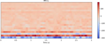
The Mel-frequency cepstral coefficient, or MFCC, is a fea-ture that allows the identification of persons based on au-dio. The technique is already used in various speech recog-nition applications. MFCC is a feature based on the Mel scale, a scale that translates measured frequency to per-ceived frequency. This means that sound is looked at in a way which humans hear it; with more emphasis at the fre-quency ranges in which speech is. In figure 2 you can see what an MFCC looks like. On the x-axis, you can see the time in seconds and on the y-axis the MFCC coefficients. For each step, the value of these coefficients is indicated by the color.
Figure 2. MFCC plot
2.2.2
ZCR
The Zero Crossing Rate, or ZCR, is a simpler feature than the MFCC and is therefore easier to compute. ”Zero-crossing rate is a measure of number of times in a given time interval/frame that the amplitude of the speech sig-nals passes through a value of zero” [13]. According to this research, a high ZCR can be associated with speech, as that causes fluctuations in amplitude leading to many zero crossings.
2.3
Support Vector Machine
In machine learning, models are used to classify data. The model we use to predict the number of speakers in an audio file is called a Support Vector Machine (SVM). The basics are that an SVM looks at the different classes (in our case, the number of speakers) and tries to differentiate among them. It does so by separating classes with a line, plane or hyperplane, depending on the number of classes. This separation is made so it has the maximum distance from each of the classes. SVM is part of supervised machine learning. This means it first needs labeled data to train on. After training the model, it can be used to predict what class new data samples belong to [5].
3.
RELATED WORK
One of the earlier researches looking into person identifica-tion by speech originates from 1995. Reynolds and Rose [9] looked at the application of Gaussian Mixture Mod-elling (GMM). When they published their paper, other approaches from that time required large and especially long datasets or took a long time to compute. They pro-posed a novel way which required clips of 10 seconds and was far more reliable in handling noise. In an experiment with 49 speakers was shown that their approach is able to identify speakers with an accuracy of 96,8% on short, clean, speech samples. On longer noisy samples the per-formance reaches 80,8% accuracy.
State of the art research regarding speaker identification from Ravanelli and Bengio [8] implements deep learning. Instead of using what they call ’hand-crafted’ features which have been used up til now, they use raw speech data. In order to do this, they use a different form of machine learning called Convolutional Neural Networks (CNN). Their model, named SincNet, is able to pick up important speaker characteristics that might be lost when only looking at certain features. SincNet trains itself to look at what audio characteristics are important for classi-fication. Compared to all other current solutions, SincNet has superior ability to identify speakers correctly. In other work, Xu et al. [15] performed research with the goal to count people using speech. A platform called Crowd++ was developed to facilitate this counting. The research focuses on a simpler solution. The counting and accompanying calculations are all performed on a smart-phone. Using unsupervised machine learning and audio data from phone microphones, they can determine the number of people in a conversation. By using an unsu-pervised approach, the need for labeled data is removed. Crowd++ takes small sections of a recording, which are analyzed by looking at the pitch and MFCC. Based on these values, Crowd++ determines if this speaker is new, or that the person has spoken before. With this approach, Crowd++ assumes that speech is not simultaneous. In bigger areas such as restaurant, one smartphone per table (conversation) is required in order to determine the total number of persons present. Possible use-cases are social sensing and personal well-being assessment.
[image:2.595.62.277.545.639.2]show that SVMs can successfully distinguish among dif-ferent classes.
4.
RESEARCH QUESTION
To minimize the costs and effort while counting people, we would like to use sensors that are currently present in office buildings. WiFi and Bluetooth tracking are not sufficient and also motion sensors are not usable for determining the number of people in a room. As an alternative to motion sensors, we will investigate the use of sound, since microphones are present in many devices. Smartphones are one example of devices that are used everywhere and include a microphone.
SVMs have shown to be able to distinguish between dif-ferent audio classes. There are current solutions that are able to identify speakers quite accurately. Crowd++ is an option that counts people and has shown to be use-ful in experiments. A downside is that it expects unique speech, meaning one person is speaking at a time. There is always the possibility of overlapping speech, therefore we will look at the application of SVM in identifying the number of speakers in simultaneous speech.
This leads to the following research questions.
RQ1Can we identify the number of simultaneous speakers by looking at sound features?
RQ1.1What features of sound can be used to count the number of simultaneous speakers?
RQ1.2 How can we adjust these features and our model for an optimal result?
5.
METHODOLOGY
In section 2 we already answered RQ 1.1 by indicating what features we will use: MFCC and ZCR. In order to train and test our model, we needed labeled data with simultaneous speakers. To get a large dataset and con-sistent results, we generated simulations in which speech was mixed together. This allowed us to quickly test many cases without having to record and label audio data our-selves. It also allowed for many different scenarios to be created. Options include a varying number of people that have a conversation, talk independently from each other or all talk at the same time. For our research, we focused on the last option: simultaneous speech.
5.1
Generate input
5.1.1
Prepare audio
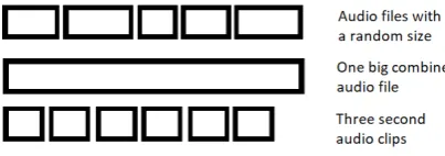
The first step is to gather audio. We used a public collec-tion of audio files. These audio files all have the same for-mat and sampling rate, eliminating a pre-processing step. Since we want to create simulations with multiple speak-ers, we first created one audio file for each speaker. From this file, we created as many short 3 second fragments as possible. See figure 3. We chose for three seconds since this frame size is also used in other literature [15] and makes sure we only need a short audio segment for clas-sification. The audio files were combined and later split up in three-second clips by using Pydub [10]. Pydub is a Python library which allows for easy manipulation of audio.
5.1.2
Creating scenarios
[image:3.595.319.521.60.131.2]With the three-second clips created, we generated differ-ent scenarios. These scenarios were used to train and test our model. In order to do this, for n speakers we ran-domly picked a speaker and one of his/her three-second clips. This resulted in a total of n random audio clips from
Figure 3. Dataset preparation
unique speakers. To simulate real environments, where some people might be further from the microphone than others, each clip was randomly made quieter. This was done by reducing the volume with a random value rang-ing from one to 10 decibel. Next, the clips were mixed together to create one scenario. For each number of si-multaneous speakers, ranging from one to 20, 700 scenarios were created to provide us with enough test and training data.
5.2
Creating a model
5.2.1
Extracting features
For each of the mixed audio clips, we first needed to ex-tract the features. To exex-tract these features, LibROSA[4] was used. LibROSA is a Python package that can be used for audio analysis. The features were then stored. This al-lowed us to do multiple runs of the model, without having to extract the features on every run.
The features we used, MFCC and ZCR, are in their orig-inal form too big to use with an SVM. Both features are represented by a number of rows and columns with val-ues. In order to compress the features, we took the mean and variance of each row of data. For MFCC, this was 15 rows, and for ZCR one. This resulted in a remainder of 30 values for the MFCC and 2 for the ZCR. The compressed version of the features was saved locally for later usage.
5.2.2
Building the SVM
We created a Python class to represent the SVM. This class receives all relevant variables, such as what data to use, how many scenarios it should use in its calculation and what the division was between train and test data. The model starts by listing all the files it receives. For each number of speakers, 70 percent is stored in the training set and the remainder in the test set. Once the train and test sets have been created, we can run the SVM. It is first fitted using the labeled training data. After this step, the test data is fed to the SVM model which returns an estimation of the number of speakers for each of the samples.
5.3
Creating a framework
Using the input generator and model we built a framework to assess the performance of our model. This framework allowed us to test multiple features, feature variables, and SVM options consecutively. Finally, the framework al-lowed us to visualize and verify the created model. Using its output we can evaluate the performance of different ma-chine learning techniques and sound features. The steps in this framework are visualized in figure 4.
6.
EXPERIMENT AND RESULTS
6.1
Dataset
Figure 4. Steps of the framework
data, originating from public domain audiobooks. The set is originally intended for training of speech detection. In total 1201 of the available speakers are female, and 1283 of the audiobooks are read by men. We used only a small subsection of the whole set called ’dev-clean’, en-suring that we have clean speech data. The set consists of 20 male and 20 female speakers. This ratio makes the division of male to female fair, preventing a bias on gen-der. In total, around 8 minutes of speech are available for every speaker. The sample rate for all data in LibriSpeech is 22050 Hz.
6.2
Experiments
We tested our model by changing a number of variables. This allowed us to get the best possible performance, after which we evaluated the system as a whole. We start by changing the variables used in the feature extraction, fol-lowed by changing the SVM c value and concluding with an evaluation of the overall performance. To evaluate our model we looked at three outputs. Accuracy, the F1 value, and a confusion matrix. The accuracy of our model is the percentage of the correct estimated number of speakers. The F1 value is a more specialized way of looking at accu-racy, taking into account precision (true positives divided by all positives) and recall (true positives and false nega-tives). A confusion matrix can be used to visualize our re-sult. On the Y-axis, the true number of speakers is shown and on the X-axis the predicted number of speakers. In a perfect scenario, this would result in one line from the top left to the bottom right.
6.2.1
MFCC variables
When extracting the MFCC using LibROSA a few vari-ables must be selected. The most relevant ones are n FFT and hop length. When creating an MFCC, a number of Fast Fourier Transformations (FFT) has to be made. The n FFT stands for how many samples (frames) are used in each FFT and thus the duration of each segment over which FFT is performed. The hop length stands for how big the steps should be before taking a new FFT. We started by varying the hop length and number of FFTs. A smaller hop length gives us more chance to catch impor-tant details, but making the hop length too small results in unusable data, as the FFT will eventually be performed for every existing frame. By varying the number of FFTs we decide for each hop how many samples we look at. The number of FFTs influences how much detail we can find in a sample. In the following experiments, we looked at Accuracy and F1. The used feature was MFCC. For our samples, we used 500 scenarios of up to 10 speakers. The used c value was 100. See figure 5 and 6. Note that the effects shown in these figures are flat. The hop length and nFFT have only minor effects on F1.
From these graphs, we find that the optimal n FFT size is 512. For the hop size there appear to be three optimums.
By looking at the F1 value we find that 64 gives the best result.
0 200 400 600 800 1,000 1,200 0.32
0.34 0.36 0.38 0.4
Hop Length Varying MFCC hop length
Accuracy (%) F1
Figure 5. F1 and Accuracy as a function of hop length
0 200 400 600 800 1,000 1,200 0.32
0.34 0.36 0.38 0.4
n FFT Varying n FFT size
[image:4.595.318.534.88.228.2]Accuracy (%) F1
Figure 6. F1 and Accuracy as a function of n FFT
6.2.2
SVM variable
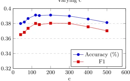
After we found the optimal values for our MFCC features, we look at the SVM variables. For an SVM, the value c indicates how much you want to avoid disqualifications. A bigger c value will give a smaller margin to the hyperplane with training data. This could lead to better accuracy, but also cause disqualifications with the test set. For these tests, we used the MFCC with a hop length of 64 and nFFT of 512. See figure 7.
0 100 200 300 400 500 600 0.32
0.34 0.36 0.38 0.4
c Varying c
Accuracy (%) F1
[image:4.595.318.533.295.436.2] [image:4.595.319.529.599.730.2]6.2.3
Different features
In this research, we mainly focused on the MFCC. To ac-company this variable we will look if adding the ZCR to the equation helps us to improve accuracy. In 8 we show their performance over 5 to 20 simultaneous speakers. On the Y-axis the average of accuracy and F1 is indicated. The combination of MFCC and ZCR performs slightly better than only MFCC, although the advantage becomes neglectable as the number of speakers increases.
5 10 15 20
0.2 0.3 0.4 0.5 0.6
Number of speakers
Comparing MFCC and MFCC + ZCR
[image:5.595.328.521.54.223.2]MFCC MFCC + ZCR
Figure 8. Average of F1 and Accuracy as a func-tion of the number of speakers
6.3
Results
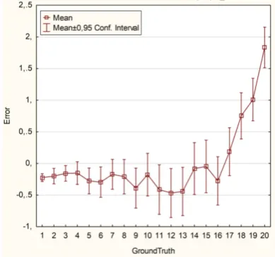
With the experiments above we were able to determine the optimal variables for the MFCC and SVM. This an-swers RQ 1.2. With our optimal variables and the MFCC and ZCR combined we achieve the following matrix for ten people with 700 samples for training and testing. See fig-ure 9. In the matrix, we can see that for a small number of speakers the estimation is accurate. As can be expected, the error in the prediction varies more if the number of speakers increases. To give an idea of the accuracy we made a plot with the mean error. Error is defined by the number of speakers (GroundTruth) minus the predicted number of speakers. This graph gives a better indication of how far off our model is on average, and might allow us to find a potential bias.
Our results show that it is possible to estimate the number of speakers with an SVM. From the confusion matrix, we can see that our model is quite accurate. This is better visualized in the error plot. Until 16 speakers our model has a slight overestimation, and from 17 on it starts to underestimate the number of speakers.
7.
DISCUSSION
7.1
Results
[image:5.595.72.272.169.303.2]The F1 and Accuracy in our experiments lies between 0.3 and 0.4. This seems like a small number, but for these values, we only look at correct and false estimations. If 20 people talked in a scenario and our model predicted 19 speakers, this is indicated as wrong. Therefore we look at the confusion matrix and mean error for our final re-sult. One remark we can see in both the confusion ma-trix and the mean error plot is that the minimum and maximum amount of speakers our model trained with are picked more often. This can be explained by the fact that our model cannot under or overestimate. Less than one speaker is not an option, and it never learned that more than 10 or 20 speakers respectively is an option. This also shows in the mean error graph. Overall our model tends to
Figure 9. 10 person confusion matrix
Figure 10. Mean error as a function of the actual number of speakers
overestimate just a little. In the end, we can see the error goes up and our model starts to underestimates the num-ber of speakers. This is as we approach 20, the maximum our model was trained on. Another note on our results is that this accuracy is an average over a lot of samples. In the matrix can be seen that some estimations are quite far off. In real life scenarios, where only one measurement is made this could pose a problem. However, at the moment we only look at a three-second interval for counting. In a real-life situation, we could do this multiple consecutive times to achieve higher accuracy.
7.2
Limitations
As with any machine learning approach, we looked only at a number of features, better results might be achieved with others. While the model we used seems to function prop-erly and the features have been proven in earlier research, other options are still available. The CNN approach used in SincNet might be able to detect simultaneous speakers instead of only speaker identification.
[image:5.595.326.521.260.442.2]loudness.
Visualizing the SVM might allow for a better idea of how it is training on the given features. It could help us to ensure we are not overfitting with the used C value, and we are not looking at features or statistics which are only relevant in our simulation. It might also facilitate a look at the effect of the MFCC and C values.
7.3
Bias
LibriSpeech provides a lot of training data. While this is convenient during the development of our model, it does limit the variety of our samples. A potential bias is lan-guage and speech. Every speaker our model is trained with speaks proper English. Other languages might have differ-ent tones or articulations. Since our model was not trained according to this, counting speakers might not work as well in these languages as it did with our training data. Test-ing and the implementation in English speakTest-ing countries should not be an issue. However, when our project should be implemented in other regions problems may arise. Cur-rent speech recognition already has problems with accents [6]. Although we do not try to recognize speech, similar problems may occur. To prevent this our model should be further trained on bigger datasets before it is used in further applications.
8.
CONCLUSION
In this research, we demonstrated a framework to classify the number of speakers during simultaneous speech using Support Vector Machines. In order to build this frame-work, we first created audio fragments for a total of 40 unique speakers. Using these files scenarios containing a variable number of unique speakers were created. These scenarios were used to train and test an SVM model. In our experiments, we looked at the MFCC and ZCR. By changing the parameters used for feature extraction we optimized our model. We also changed the c value our SVM used to find an optimum. The Zero Crossing Rate appears to only have a marginal added value in identifying a number of speakers.
Finally, we show that using our model an accurate predic-tion of the number of simultaneous speakers can be given. Until 17 speakers the mean error only deviates a maximum of 0,5 person. We do have to note that these numbers are on average. To achieve higher accuracy on individual cases multiple consecutive measurements can be taken. In most use cases the exact number of people is not relevant, an in-dication would be sufficient. Additionally, our framework could be deployed in combination with existing systems that count people, to achieve increased accuracy and con-fidence.
For future work, there are many areas in which this re-search could be expanded. There are many more promis-ing features which could be tested our data. Different scenarios could be created, with more lifelike situations in which simultaneous speech occurs. Possibilities include different settings by adding background noise from an of-fice or street environments. Different ways people inter-act, for example, conversations between groups of people. Another option is to use more challenging parts of the Lib-riSpeech dataset or use completely different datasets alto-gether. Finally, it might be worth to investigate the use of other machine learning techniques. Especially the
ap-proach using Convectional Neural Networks, as done with SincNet [8] could be promising.
9.
REFERENCES
[1] K. Baldauf.Succeeding with Technology (Available Titles Skills Assessment Manager (SAM) - Office 2010). Course Technology, mar 2008.
[2] G. Guo and S. Z. Li. Content-based audio classification and retrieval by support vector machines.IEEE transactions on Neural Networks, 14(1):209–215, 2003.
[3] L. Mainetti, L. Patrono, and I. Sergi. A survey on indoor positioning systems. In2014 22nd
International Conference on Software, Telecommunications and Computer Networks (SoftCOM), pages 111–120. IEEE, 2014. [4] B. McFee, C. Raffel, D. Liang, D. P. Ellis,
M. McVicar, E. Battenberg, and O. Nieto. librosa: Audio and music signal analysis in python. In Proceedings of the 14th python in science conference, pages 18–25, 2015.
[5] D. Meyer and F. T. Wien. Support vector machines. The Interface to libsvm in package e1071, page 28, 2015.
[6] D. Mitrovi´c, M. Zeppelzauer, and C. Breiteneder. Features for content-based audio retrieval. In Advances in computers, volume 78, pages 71–150. Elsevier, 2010.
[7] V. Panayotov, G. Chen, D. Povey, and
S. Khudanpur. Librispeech: an asr corpus based on public domain audio books. In2015 IEEE
International Conference on Acoustics, Speech and Signal Processing (ICASSP), pages 5206–5210. IEEE, 2015.
[8] M. Ravanelli and Y. Bengio. Speaker recognition from raw waveform with sincnet. In2018 IEEE Spoken Language Technology Workshop (SLT), pages 1021–1028. IEEE, 2018.
[9] D. A. Reynolds and R. C. Rose. Robust text-independent speaker identification using gaussian mixture speaker models.IEEE transactions on speech and audio processing, 3(1):72–83, 1995. [10] J. Robert. Pydub by jiaaro, Jan 2011.
[11] J. Scheuner, G. Mazlami, D. Sch¨oni, S. Stephan, A. De Carli, T. Bocek, and B. Stiller. Probr-a generic and passive wifi tracking system. In2016 IEEE 41st Conference on Local Computer Networks (LCN), pages 495–502. IEEE, 2016.
[12] D. Sharp. What is sound?, Feb 2017.
[13] D. Shete, S. Patil, and S. Patil. Zero crossing rate and energy of the speech signal of devanagari script. IOSR-JVSP, 4(1):1–5, 2014.
[14] F. Wahl, M. Milenkovic, and O. Amft. A distributed pir-based approach for estimating people count in office environments. In2012 IEEE 15th
International Conference on Computational Science and Engineering, pages 640–647. IEEE, 2012. [15] C. Xu, S. Li, G. Liu, Y. Zhang, E. Miluzzo, Y.-F.