Using generalized linear models to model compositional response data

(1)

warwick.ac.uk/lib-publications

A Thesis Submitted for the Degree of PhD at the University of Warwick

Permanent WRAP URL:

http://wrap.warwick.ac.uk/89876

Copyright and reuse:

This thesis is made available online and is protected by original copyright.

Please scroll down to view the document itself.

Please refer to the repository record for this item for information to help you to cite it.

Our policy information is available from the repository home page.

(2)

USING GENERALIZED LINEAR MODELS TO MODEL

COMPOSITIONAL RESPONSE DATA

by

Fiona Sammut

A thesis presented for the degree of

Doctor of Philosophy

Department of Statistics

University of Warwick

(3)

Dedication

(4)

List of Figures

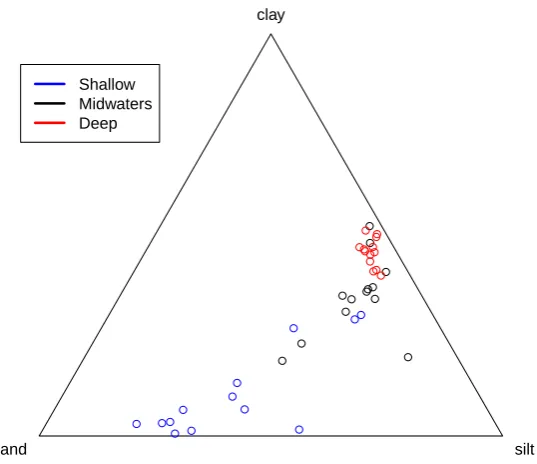
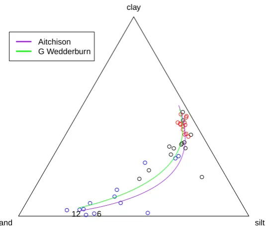
3.1 A Ternary Diagram showing Arctic Lake Compositional Data in Relation to Depth . . . 101 3.2 A Ternary Diagram showing the fitted lines achieved under Aitchison’s

ap-proach and Generalized Wedderburn apap-proach using the Arctic Lake Dataset103 3.3 Cook’s Distances Plots obtained using Aitchison’s approach for the Arctic

Lake Dataset . . . 104 3.4 Plots of Generalized Wedderburn Residuals fitted against Log Depth for

the Arctic Lake Dataset . . . 104 3.5 Plots of Aitchison Residuals fitted against Log Depth for the Arctic Lake

Dataset . . . 105 3.6 Normal QQ Plot of Generalized Wedderburn Residuals for the Arctic Lake

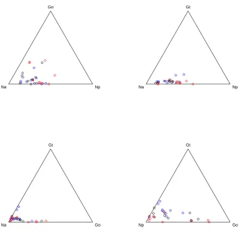
Dataset . . . 106 3.7 Normal QQ Plot of Aitchison Residuals for the Arctic Lake Dataset . . . . 106 3.8 A Matrix of Ternary Diagrams for the Foraminiferal Subcompositions in

Relation to Depth . . . 109 3.9 Plots of Generalized Wedderburn Residuals fitted against Depth for the

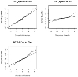
Foraminiferal Dataset . . . 112 3.10 Plots of Aitchison Residuals fitted against Depth for the Foraminiferal Dataset113 3.11 Normal QQ Plot of Generalized Wedderburn Residuals for the Foraminiferal

Dataset . . . 114 3.12 Normal QQ Plot of Aitchison Residuals for the Foraminiferal Dataset . . . 114 3.13 A Ternary Diagram showing the Fitted Lines achieved for the

Subcompo-sitions of Np, Go and Gt, using the Generalized Wedderburn Model and Aitchison’s Model for the Foraminiferal Dataset . . . 115 3.14 A Ternary Diagram showing the Fitted Lines achieved for the

Subcompo-sitions of Na, Np and Go, using the Generalized Wedderburn Model and Aitchison’s Model for the Foraminiferal Dataset . . . 115

(9)

E.1 Ternary Diagrams of the First Generated Sample of Size 60 assuming dif-ferent Correlations and Coefficients of Variation . . . 145 E.2 Ternary Diagrams of the First Generated Sample of Size 180 assuming

different Correlations and Coefficients of Variation . . . 146 E.3 Ternary Diagrams of the First Generated Sample of Size 600 assuming

different Correlations and Coefficients of Variation . . . 147

F.1 Scatter Plots of Generalized Wedderburn versus Aitchison Estimates using a simulation size of 105_{, samples of size 60, assuming independence, and}

coefficients of variation (5%,5%,20%) and (30%,30%,60%) in the upper and lower panes respectively . . . 149 F.2 Scatter Plots of Generalized Wedderburn versus Aitchison Estimates using

a simulation size of 105_{, samples of size 60, assuming correlation 0.3, and}

a simulation size of 105_{, samples of size 180, assuming independence, and}

a simulation size of 105_{, samples of size 600, assuming independence, and}

(10)

F.9 Scatter Plots of Generalized Wedderburn versus Aitchison Estimates using a simulation size of 105_{, samples of size 600, assuming correlation 0.7, and}

(11)

List of Tables

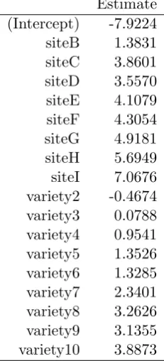
2.1 Barley Leaf Data Parameter Estimates . . . 41

3.1 Table of True γ Parameters . . . 84 3.2 Table of Estimated Bias and Standard Error of the Bias achieved under

Aitchison and Generalized Wedderburn Approach using a sample of size 60 assuming independence, correlation of 0.3 and correlation of 0.7 and a simulation size of 105 _{. . . 88}

3.3 Table of Estimated Bias and Standard Error of the Bias achieved under Aitchison and Generalized Wedderburn Approach using a sample of size 180 assuming independence, correlation of 0.3 and correlation of 0.7 and a simulation size of 105 _{. . . 89}

3.4 Table of Estimated Bias and Standard Error of the Bias achieved under Aitchison and Generalized Wedderburn Approach using a sample of size 600 assuming independence, correlation of 0.3 and correlation of 0.7 and a simulation size of 105 _{. . . 90}

3.5 Table of Variance Estimates together with their standard errors achieved under Aitchison and Generalized Wedderburn Approach using a sample of size 60 under independence, correlation of 0.3 and correlation of 0.7 and a simulation of size 105 _{. . . 93}

(12)

3.9 Table of Variance Estimates together with their standard errors achieved under the Generalized Wedderburn Approach using a sample of size 180 assuming independence, correlation of 0.3 and correlation of 0.7 and a sim-ulation of size 105_{. . . 97}

3.10 Table of Variance Estimates together with their standard errors achieved under the Generalized Wedderburn Approach using a sample of size 600 assuming independence, correlation of 0.3 and correlation of 0.7 and a sim-ulation of size 105_{. . . 98}

3.11 Table of Coverage Probabilities achieved under the Generalized Wedder-burn Approach using both model-based and robust variance estimators with samples of size 60, 180 and 600 under three different correlations and a sim-ulation of size 105_{. . . 99}

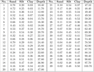
3.12 The Arctic Lake Dataset . . . 100 3.13 Table of Estimates and their Standard Errors Obtained using Aitchison’s

approach and the Generalized Wedderburn approach on the Arctic Lake Dataset . . . 102 3.14 Table of Distance Measures achieved using Aitchison’s approach and the

Generalized Wedderburn approach on the Arctic Lake Dataset . . . 102 3.15 The Foraminiferal Dataset with Proportions: Na: Neogloboquadrina

At-lantica, Np: Neogloboquadrina Pachyderma, Go: Globorotalia Obesa, Gt: Globigerinoides Triloba . . . 108 3.16 Table of Estimates and their Standard Errors Obtained using the

General-ized Wedderburn approach on the Foraminiferal Dataset Without Imputation110 3.17 Table of Estimates and their Standard Errors Obtained using Aitchison’s

approach and the Generalized Wedderburn approach on the Foraminiferal Dataset With Imputation . . . 110 3.18 Table of Distance Measures achieved using Aitchison’s approach and the

Generalized Wedderburn approach on the Foraminiferal Dataset . . . 111

4.1 Table of Estimates and their Standard Errors Obtained from fitting a Dirichlet Regression Model to the Arctic Lake Dataset . . . 119 4.2 Table of Estimates, Estimated Bias and Estimated Standard Error of the

Bias achieved using MLE and GEE on Dirichlet simulated data based on estimates from the Arctic Lake dataset with a sample of size 39 and a simulation of size 105 _{. . . 121}

(13)

(14)

Acknowledgements

Without the help and support of a number of people, this work would not have been possible. In particular, I wish to thank:

My supervisor, Professor David Firth whose knowledge, guidance, stimulating suggestions and constructive criticism helped me throughout the different stages of preparing this thesis.

My friends Monique, Stephanie, David, Natalie and Shirley for their ever encouraging words and support.

Elena, Silvia, Panayiota and Pantelis for their friendship and for making me feel at home away from home.

My family whose thoughtful words made me a stronger person.

Especially, I would like to thank my husband, Trevor, for believing in me and supporting me through the good and the bad and whose patient and unconditional love enabled me to complete this work.

(15)

Declaration

(16)

Abstract

(17)

List of Notation

˙

Y vector of latent variables

Y composition

W vector of logratios

J number of components inY and ˙Y

Yj jth component in Y X design matrix

Xi design matrix corresponding to casei Xk kth explanatory variable

SJ−1 (J−1)-dimensional unit simplex

RJ J-dimensional Euclidean space

RJ+ the positive orthant ofJ-dimensional Euclidean spaceRJ

C(·) closure operation

β vector of model coefficients

γ identifiable vector of model coefficients θi, ˙θi nuisance parameters for casei

mi(θ,β) a function defined by exp

θ+x0_iβ

pij proportion for caseiand compositional variablej

p_i vector of proportions (pi1, . . . , piJ) for case i

Pi diagonal matrix with proportions (pi1, . . . , piJ) for case i φ dispersion parameter

ωj relative dispersion parameter corresponding to componentj

Ω diagonal matrix of relative dispersion parameters α_jj0 the correlation between ˙Y_ij and ˙Y

ij0 W working correlation matrix

U vector of estimating equations ˙

D matrix of derivatives ofmi

˙ θi,βj

with respect toβ and θ 1 vector of ones

110 matrix of ones

I identity matrix

Vpi,Ω,W working variance-covariance matrix used under the generalized

Wedderburn method

Vi implied form of the variance-covariance matrix ofYi A⊗B the kronecker product of matrixAwith matrix B F matrix of contrasts

Ψ variance-covariance matrix of logY˙

(18)

List of Abbreviations

GEE Generalized Estimating Equations GLM Generalized Linear Model

GLS Generalized Least Squares GW Generalized Wedderburn ML Maximum Likelihood

(19)

Chapter 1

Introduction

This thesis concerns regression modeling of compositional data, that is, models and asso-ciated methods used to describe the dependence of compositional responses upon explana-tory variables. This chapter aims to provide the setting required, to better appreciate the challenges that have been faced in trying to find a suitable approach to model continuous compositional data. An introductory note on what compositional data is, is provided in Section 1.1. Section 1.2 then gives some details on a number of distributions that have been considered apt to model this type of data, namely the Dirichlet distribution and some of its generalizations, and the logistic normal distribution. The normal distribution, Barndorff-Nielsen and Jørgensen (1991) simplex distribution, the von Mises distribution and the Kent distribution (Kent, 1982) are also mentioned briefly. The logratio trans-formation (Aitchison, 1982) is presented in relation to the logistic normal distribution. Through this transformation it is possible to model the influence of explanatory variables on the transformed variables, using standard multivariate techniques. The main drawback with the logratio transformation is that it fails when any zeros are present in the data. A brief account of various ways in which researchers have tried to tackle the problem of zeros is thus provided in Section 1.3. Section 1.4 then describes some previous attempts at modeling compositional response data through the generalized linear modeling frame-work. Studies which used the method of generalized estimating equations (GEE) to model compositional response data are presented in Section 1.5. At the end of Section 1.5, a new approach which may be used to model continuous compositional response variables and which will be developed in this thesis, is introduced. This approach is also based on the technique of generalized estimating equations.

1.1 What is Compositional Data?

(20)

of how a composition may arise include measurements on the mineral and chemical content of rocks, household expenditure patterns, or time allocated to various activities during a particular day.

Due to the nature of compositional data, one part of the composition may always be written in terms of the remaining parts, effectively reducing the dimension of a J-part composition to J−1. The importance thus lies not with the actual value of a part in a composition but with the magnitude of a part in relation to the magnitude of the other parts in a composition. In much of the theoretical development of compositional data, the magnitude of the constant k in the sum-constraint, is set equal to 1. Fixing k at 1 gives rise to a (J−1)-dimensional unit simplex, SJ−1, embedded in a J-dimensional non-negative space. Without loss of generality, the material presented in this work will take k to be equal to 1.

Let ˙Y be aJ-vector in the positive space IRJ

+, defined as ˙Y=

˙

Y1, . . . ,Y˙J

0

, where each ˙

Yj (j= 1, . . . , J), is measured in the same units and each ˙Yj provides relative information. The term relative refers to the fact that meaning to the information provided is given by the ratios of the different components. Due to only relative information being provided by the data, the unit of measurement chosen for ˙Ywill make no difference to the analysis. In fact, any two such vectors, say ˙Yand ˙Y∗, which are related by the equation ˙Y∗=aY˙, for some positive constant a, are regarded as equivalent. The equivalent vectors ˙Y∗ and

˙

Ymay both be said to fall into the class clY˙=naY˙ :a >0o, the latter geometrically

represented by a ray from the origin in IRJ

+. Intersecting this ray and the unit simplexSJ−1

results in any vector in the class cl

˙

Y

to be sum-constrained to 1. This intersection,

a constraining operation known as closure, relates the compositionY to any vector ˙Y in classcl

˙

Y

as follows

Y=CY˙= Y˙

˙

Y1+· · ·+ ˙YJ

. (1.1)

The fact that a whole class of vectors in IRJ

+ have the same closure Y leads to

prob-lems in analyzing compositional data using standard multivariate techniques directly. In particular, as per Aitchison (1986), the independence of the components of ˙Y would not correspond to any simple ‘null’ structure of the covariance between the components of the compositionY. Restriction on the variance-covariance structure of the variables form-ing the composition arises in the fact that at least one covariance is forced, through the sum constraint, to be negative. As an example of the latter, consider J = 2 and the sum constraint Y1 +Y2 = 1. From this it follows that Cov (Y1, Y1+Y2) = 0 and hence

Var (Y1) =−Cov (Y1, Y2) automatically. This restriction on Cov (Y1, Y2) will then lead to

a restriction in the correlation coefficient.

(21)

com-positional data. Nothwithstanding this fact, scientists and statisticans alike still resorted to the standard multivariate techniques to analyze this type of data and it was only around the 1960s that papers which expressed disapproval towards using the usual statistical ap-proach started to emerge.

The most prominent critic of the time was the geologist Felix Chayes. His criticism was mainly focused on the interpretation of the correlation coefficient between components in a geochemical composition. Chayes (1960) stated ‘neither the resulting spurious correlation itself nor the difficulty it creates with regard to the interpretation of composition data has been adequately described, and no general remedy has yet been suggested’.

A lot of effort has been directed in trying to obtain a formulation for this spurious cor-relation, or mostly known as null correlation as opposed to the zero correlation resulting from lack of dependence in the usual statistical sense. Papers by Darroch (1969), Meisch (1969), Darroch and Ratcliff (1970), Darroch and Ratcliff (1978) and Kork (1977), all dealt with the issue of the sum-to-a-constant constraint and its relation to the interpretation of correlations of proportions. Aitchison (1984) still felt the need to encourage researchers, petrologists in particular, to apply the right methodology in dealing with compositional data. Illustrations and warnings on why standard statistical techniques would fail had been issued back then, but were largely disregarded.

According to Aitchison (1982, 1984a), it was the ‘lack of concepts of independence, lack of a satisfactory and interpretable covariance structure and the lack of parametric classes of distributions’ which were appropriate for the simplex, that hindered the development of suitable methods for such data. To this end, Aitchison (1986) and Pawlowsky-Glahn and Egozcue (2006) recognized the fact that until the early 1980s there was no clear guidance on how to deal with compositional data.

1.2 In Search of a Family of Suitable Distributions

1.2.1 The Dirichlet Distribution

Prior to the 1980s, the only familiar class of distributions which was thought to be ap-propriate for the space of all continuous compositions was the Dirichlet family, which is defined as follows:

Definition 1.2.1. Let Y= (Y1, . . . , YJ)0 where YJ = 1− J−1

X

j=1

Yj and letα= (α1, . . . , αJ)0

∈ IRJ₊. Y is said to follow the Dirichlet distribution on SJ−1 with parameter α if its probability density function is given by

f(y1, . . . , yJ−1|α) =

Γ (α1+· · ·+αJ)

QJ

j=1Γ (αj) J

Y

j=1

yαj−1

(22)

where (y1, . . . , yJ)0 denotes a vector of values of (Y1, . . . , YJ)0 and yj ∈(0,1).

Letting α+=α1+· · ·+αJ, some well known properties of the Dirichlet distribution are

E(Yj) = αj α+

, (1.3)

Var (Yj) =

αj(α+−αj) α2₊(α++ 1)

, (1.4)

and for j6=j0

CovYj, Y_j0

= −αjαj

0

α2₊(α++ 1)

(1.5)

CorrYj, Y_j0

=−

v u u t

αjα_j0

(α+−αj)

α+−α_j0

. (1.6)

Gueorguieva et al. (2008) and Maier (2014) are examples of researchers that have used Dirichlet regression models to model compositional response variables. Focusing on (1.5) and (1.6), it may however be noted that the correlation structure of the Dirichlet distri-bution is completely negative. The Dirichlet distridistri-bution would thus not be able to cater for non-negative correlations in the data, should any be present.

Also, the Dirichlet distribution inherits an independence structure through its own def-inition. Correlations between components (Y1, . . . , YJ) arise solely through the closure operation. As per Aitchison (1982), if a composition Y is assumed to follow a Dirichlet distribution, thenYmay be considered to be the result of a closure operation performed on independent gamma distributed random variables, each having the same scale parameter.

(23)

tractability than the generalized Liouville distribution’ (Rayens and Srinivasan, 1994). Migliorati et al. (2016) also state that through its mixture structure, the flexible Dirichlet distribution may be used to model various features of a compositional data set, ‘including unimodal and multimodal cases’. However Migliorati et al. (2016) recommend to develop ‘more flexible structured mixture models’ which are ‘still inferentially tractable’.

1.2.2 The Logistic Normal Distribution

As an alternative to modeling the compositional data directly in the simplex, a parametric class of distributions which could cater for the dependence structure between the parts of the compositions but which could also make the transition from the the positive real line to the whole real line possible was devised. McAlister (1879) realized that if he consid-ered a normally distributed random variable, by taking its exponent, a useful distribution (the lognormal) would be induced on the positive real line. Throughout the 20th cen-tury, especially following the work on variance-stabilizing transformations for analysis of variance, the general Box-Cox transformation (Box and Cox, 1964) and other work on transformations to normality continued to emerge. In spite of this, it was only in the early 1980s that a new method based on McAlister’s (1879) idea of inducing a distribution on an ‘awkward’ space, from another distribution defined on a more familiar space, by using a transformation between the two spaces, was devised.

Prior to the 1980s, the logistic-normal distribution had already been used in areas like Bayesian analysis for the description of a prior and posterior distribution of multino-mial probabilities (Lindley, 1964), logistic disciminant analysis (Anderson, 1972) and in analyzing binary data. The application of the logistic-normal distribution to the field of compositional data is attributed to Aitchison and Shen (1980). As per Aitchison and Shen (1980), if the logistic transformation is applied to a (J−1)-vector W∈IRJ−1, whereW

follows the multivariate normal distribution, the resulting vector may be said to follow a logistic-normal distribution.

Definition 1.2.2. ForY∈SJ−1 andW ∈IRJ−1, the generalized logistic transformation,

also known as the additive logistic transformation, is given by

Yj =



 

 

exp(Wj)

1+PJ−1

j0=1exp

W

j0

if j= 1, . . . , J−1

1

1+PJ−1

j0=1exp

W

j0

if j=J,

where for j = 1, . . . , J −1, its inverse function is given by

Wj = log

Yj YJ

. (1.7)

(24)

So as to overcome the problem of analyzing compositional data, Aitchison (1982) proposed the use of logratio transformations, amongst which is the additive logratio transformation. If the multivariate normal distribution may be shown to be a reasonable approximation to the distribution of the logratiosW1, . . . , WJ−1, conventional multivariate techniques may

be used on the logratio-transformed data and standard statistical analysis may then be carried out in the real space IRJ−1_{. Aitchison (1982) used this idea to model the influence}

of explanatory variables X1, . . . , Xp on compositional response variables: for a sample of sizenand J components,

E

log

Yij YiJ

=x0_iβ_j (1.8)

wherei= 1, . . . , n,j= 1, . . . , J−1,β_j is a (p+ 1)-vector of coefficients which need to be estimated and xi is a (p+ 1)-vector of observations with xi0 = 1 since the first element

corresponds to the intercept and the remaining elements correspond to the observations obtained by theith case in the sample onX1, . . . , Xp.

The method of modeling the conditional expectation of logratios is appealing for a number of reasons, including the fact that it is permutation invariant. So if any component other than YJ is chosen as the reference component in the additive logratio, the same results will be obtained (Aitchison, 1986, p. 96). As per Aitchison (1986, p. 96), standard multivariate statistical procedures are all invariant under the group of permutations of the parts 1, . . . , J of the composition.

Statisticians seemed to accept such methodology. However, transformation resistance syndrome, as described by Aitchison (2003a), especially amongst the geological community (refer to letters to the Editor of Mathematical Geology over the period 1988 to 2002; Rehder and Zier (2001); Aitchison and Barcel´o-Vidal (2001)), still prevailed. Some of the arguments brought up dealt with the theoretical nature of the subject. Others dealt with the difficulty in interpreting the transformed data.

(25)

1.2.3 Other Distributions

1.2.3.1 The Normal Distribution

After searching the literature using key words such as ‘percentage, proportion and fraction’, Kieschnick and McCullough (2003) found that the majority of researchers used the normal distribution as the conditional distribution of 2-part compositional data given a set of explanatory variables. Since compositional data is not defined over the whole real line, though, it can never follow a normal distribution.

Other attempts at using the normal distribution to analyze compositional data have also been made through the use of latent variable models. Some detail and criticism on a censored normal model and on the Butler and Glasbey (2008) latent Gaussian model will be given in Section 1.3.2.3.

1.2.3.2 Barndorff-Nielsen and Jørgensen (1991) Simplex Distribution

Another distribution which has been used to model 2-part compositional data is the uni-variate simplex distribution (Barndorff-Nielsen and Jørgensen, 1991). The density function of a response variable Y which follows a univariate simplex distribution is given by

f y|µ, σ2

= r 1

2pσ2h_y₍₁₋_y)3i

exp

− 1

2σ2d(y;µ)

,

for 0 < y < 1, 0 < µ < 1 and where d(y;µ) = (y−µ)2/y(1−y)µ2(1−µ)2 is the unit deviance. The form of the density of the univariate simplex distribution implies that the simplex distribution is a proper dispersion model (see Jørgensen, 1986) where the parameters µ and σ2 correspond to the position and dispersion parameters. This distribution is however defined on the open interval (0,1), excluding the possibility of analyzing compositional data with zeros.

In Section 1.5, we will see how the Barndorff-Nielsen and Jørgensen (1991) simplex distri-bution has been used in a generalized linear modeling setup in attempt to model compo-sitional data. Zhang (2013) made use of a multivariate version of this distribution, which is however also not suitable to model zeros in compositional data. More details on the use of the multivariate simplex distribution Barndorff-Nielsen and Jørgensen (1991) in Zhang (2013) will also be given in Section 1.5.

1.2.3.3 Distributions Defined on the Hypersphere

(26)

been used to model compositional data. More specifically, the two distributions have been used by Scealy and Welsh (2011) and Stephens (1982) respectively, to model data defined on the hypersphere. In directional data, a direction in J dimensions may be represented by a vector, sayS, which lies on the surface of a (J−1)-dimensional hypersphere of unit radius and is centred at the origin. Vectors on the surface of the hypersphere satisfy

S0S=1. Compositional data is turned into directional data by means of the square root transformation, that is by letting S = √Y1, . . . ,

√ YJ

. By the sum-to-1 constraint of compositional data,S0S=1follows naturally.

Stephens (1982) used the von Mises-Fisher distribution to discriminate between two groups of students. Aitchison (2008) acknowledges the fact that a ‘reasonable discrimination’ has been achieved on using such an approach but discourages further use of such an approach due to the simplex and the sphere being ‘topologically completely unrelated’. Mardia (1976) also showed that the von Mises-Fisher distribution can provide a good approxi-mation to the multinomial distribution, showing that the von Mises-Fisher distribution inherits the restrictive correlation structure of the multinomial distribution, making the von Mises-Fisher distribution unfit to model compositional data.

As per Scealy and Welsh (2011), the Kent distribution on the other hand, provides a ‘natural generalization’ on the von Mises-Fisher distribution, has as many parameters as the (J −1)-variate normal distribution, and its parameters are ‘readily interpretable’. Some more detail on how Scealy and Welsh (2011) have successfully managed to use the Kent distribution to model the influence of explanatory variables on compositional response variables will be given in Section 1.3.2.4.

1.3 Analyzing Compositional Data with Zeros

Compositions with zero values may easily turn up in practice. An example which is very frequently used in the literature is that of household expenditure where some families would spend nothing on alcohol and cigarettes. Zeros might also be obtained in an analysis of time allocated to different tasks with some people allocating no time to physical activity. Furthermore, zeros might also result in an analysis of the proportion of fat, carbohydrates and protein in food items, with no protein or fat found in sugar. It might also be of interest to study the presence of various species in an area with some species remaining undetected.

1.3.1 Rounded and Essential Zeros

(27)

may be considered as having been erroneously recorded as zeros (Palarea-Albaladejo et al., 2007). When this type of zero arises it is referred to as arounded zero. Aitchison (1986, p. 268) proposed to investigate ways in which rounded zeros in compositional variables may be replaced by some small positive value which is smaller than the smallest recordable value. Various imputation methods for rounded zeros, amongst which are the multiplica-tive replacement technique (Mart´ın-Fern´andez et al., 2003) and the modified EM algorithm (Palarea-Albaladejo and Mart´ın-Fern´andez, 2008) exist in the literature. So once the zeros in the data have been imputed, a logratio transformation may then be applied and the transformed data is then analysed using standard statistical techniques.

Imputation may not however be used when there are essential zeros in the data. An essential zero in a composition is a zero which may not be considered to be the result of a limitation of the measuring instrument being used but is the result of something that is completely absent. An essential zero might be obtained, for example, from a family whose expediture on household appliances during a study period is nil. In some cases, it might make sense to overcome modeling problems due to essential zeros by performing a separate analysis of subjects/objects coming from different groups/subpopulations. Alternatively, it might also be reasonable to amalgamate the proportions from different components of the composition. After amalgamation of the different parts, statistical analysis may then be carried out on the full dataset. Models that deal with the essential zero problem have been proposed but at this stage there is still no standard procedure which should be implemented.

1.3.2 Various Attempts at Solving the Essential Zero Problem

1.3.2.1 The Addition of a Constant to Every Observation

The first attempt at solving the essential zero problem came from Aitchison (1986). Aitchi-son (1986, p. 271) proposed to take insight from the three-parameter lognormal model (Aitchison and Brown, 1957) where a constant υj, j = 1, . . . , J, known or to be esti-mated is added to every observation and the logratio transformation is then applied to the vectorC(Y+υ) rather than toC(Y). Clearly, for a dataset with a large number of zeros, this technique will lead to substantial computational effort. Furthermore, even with compositions with a relatively small number of parts, with the inclusion of υj, a serious interpretation problem of the transformed data arises.

1.3.2.2 Conditional Modeling

(28)

then (1−p). Conditional on Y1 = 0, the distribution for Y(1) = (Y2, . . . , YJ)0 is taken to be the additive logistic normal distribution with parameters µ₀ and Σ0. Conditional

on Y1 >0, Y is taken to follow an additive logistic normal distribution with parameters

µand Σ. Let fJ−1(· |µ,Σ) denote the probability density function corresponding to Y.

The contribution to the likelihood by a compositional vector with Y1 = 0 is then

pfJ−2(· |µ0,Σ0)

and the contribution to the likelihood by a compositional vector with Y1 >0 is given by

(1−p)fJ−1(· |µ,Σ).

Estimation of the parameters may then be carried out through maximum likelihood esti-mation.

The setup provided by Aitchison (1986) is however a very simple one. Bacon-Shone (2003) explains that a suitable model is one which is able to handle two problems; the first being that of modeling the pattern of zeros for multiple components and the second being that of modeling a composition conditional on the particular pattern of zeros which arises. Aitchison and Kay (2003), Zadora et al. (2010) and Tsagris (2014) also propose to use a two-step approach to model compositional data with zeros. Zadora et al. (2010) and Tsagris (2014) first model the presence of zeros using the independent binary model

J

Y

j=1

puj

j (1−pj)1−uj,

wherepj is the probability of obtaining a non-zero value in thejthcomponent anduj is an indicator function taking the value 1 if thejthcomponent in a composition is not zero and a value of 0 in the presence of a zero. A multivariate density function which incorporates the model for the zeros in then adopted in the second stage.

In relevance to the nature of compositional data, the assumption of independence in the independence binary model is completely violated. Aitchison and Kay (2003) thus impose a hierarchical prior on the binomial parameters pj,

pj =

exp (λj) exp (λj) + 1

,

(29)

1.3.2.3 The Latent Model

Alternative attempts at modeling compositional data with zeros involved the use of latent variable models. The Tobit model and Butler and Glasbey (2008) latent Gaussian model are two such examples. Both models may be used in the presence of zeros. Both of them, however, are not suitable to model compositional data. More detail about the two models follows.

The Tobit Model

There are occasions (e.g. Agnew et al., 1995; Barclay and Smith, 1995) where the cen-sored normal model, also known as the Tobit model, has been used to model continuous proportions. Continuous proportions may be viewed as 2-part compositional data. For a dataset of size n, in a Tobit model, a latent (unobservable) variable ˙Y is related to p

independent variables X1, . . . , Xp, through the linear model

˙

Yi=x0iβ+Ei, i= 1, . . . , n

and the response variable Y satisfies

Yi =



 

 

0 if ˙Yi ≤0 ˙

Yi if 0<Y˙i <1 1 if ˙Yi ≥1

where β is a vector of unknown regression parameters and Ei are error terms which are assumed to be independent and identically N 0, σ2

distributed.

This model may handle zeros in the data but values outside the range (0,1) are being treated as if they were censored. It is due to the nature of compositional data that values beyond the range [0,1] may never be observed.

Butler and Glasbey (2008) Latent Gaussian Model

Butler and Glasbey (2008) propose to handle zeros in compositional data by means of a latent Gaussian model. This model is based on the assumption that compositional data is obtained through performing a transformation on an underlying set of latent variables

˙

Y. These latent variables are assumed to follow a multivariate Gaussian distribution with unknown parametersµand Σ, and ˙Y is also assumed to lie on the unit hyperplane HJ =

n

˙

y∈RJ : ˙y

0

1= 1o. Such an assumption on ˙Y implies that the mean vector µ

and the variance-covariance matrix Σ of ˙Y must satisfy µ01 = 1 and Σ110 =O, where

(30)

usual sum constraint and non-negativity of the parts of the compositions. The function performs a Euclidean projection from a unit hyperplane onto a unit simplex. Butler and Glasbey (2008) explain that the choice of the Euclidean transformation was motivated by its wide use and its pleasing theoretical properties.

The assumption that the latent variables following a multivariate normal distribution makes the estimation process relatively easy for J ≤3 but the authors acknowledge that parameter estimation becomes complicated once J > 3. Also, by assuming that the compositional data comes into existence through the multivariate normal distribution, the principles of scale invariance and subcompositional invariance are violated. The principle of scale invariance requires that any function of compositional data should be expressed in terms of ratios and the principle of subcompositional invariance requires that the same information is obtained from the components which are common to different subsets of a composition. Butler and Glasbey (2008) thus recommend that this approach is only used if i) other methods are not available or if they are inappropriate, ii) as a diagnostic tool for assessment of other methods or iii) for exploratory purposes. Butler and Glasbey (2008) also suggest to investigate the possibility of using alternative transformations.

1.3.2.4 The Square-Root Transformation

Scealy and Welsh (2011) propose an alternative approach to handle zeros in compositional data. A brief mention of this approach has also been given in Section 1.2.3.3. It is based on applying the square root transformation on compositional data, including zeros in the data, so that compositional data is transformed to directional data. Stephens (1982) and Scealy and Welsh (2011) used the square root transformation as a first step in their analysis to model compositional data. Scealy and Welsh (2011) proceed to develop a regression model for compositional data through the Kent distribution (Kent, 1982), by relating the mean direction vector to linear functions of the explanatory variables. The performance of the estimation procedure described in Scealy and Welsh (2011) is however impaired if the majority of the transformed data is close to the boundaries of the positive orthant. So Scealy and Welsh (2014) revise the estimation procedure described in Scealy and Welsh (2011) and also show how the EM algorithm may be used to estimate the parameters of the folded Kent distribution so as to deal with the problem of having a large concentration of points close to the boundaries with a ‘relatively large variance’. The Kent regression model as a means to model compositional data with zeros is promising but it lacks simplicity of implementation.

1.3.2.5 The α-Transformation

(31)

(Aitchison, 1986, p. 120).

For a composition Y and any real number α, the power transformation proposed by Aitchison (1986) is given by

S= Y

α

1

PJ

j=1Yjα

, . . . , Y α J

PJ

j=1Yjα

!0

. (1.9)

The α-transformation is then defined by

T= 1

αH(JS−1), (1.10)

where 1 is a J-dimensional vector of ones and H is the (J−1)×J Helmert submatrix

(Lancaster, 1965), the latter ‘obtained by removing the first row from the Helmert matrix’ (Tsagris et al., 2011).

Tsagris (2015) proposes an approach involving the α-transformation to model composi-tional response variables, even in the presence of zeros. Tsagris (2015) calls this method α-regression.

The steps inα-regression start by assuming that, for each case i, the conditional expecta-tion of the composiexpecta-tional response variables are given by

µij =



  

  

1

1+PJ

j0=1exp

x0_iβ j0

forj = 1

expx0_iβj

1+PJ

j0=1exp

x0_iβ j0

forj = 2, . . . , J .

The use of the multinomial logistic function ensures that, for eachi, J

X

j=1

µij = 1.

The conditional means and the compositional response variables for each i are then α-transformed to get

Yiα =

1 αH J

Y_iα₁

PJ

j=1Yijα

−1, . . . , J Y α iJ

PJ

j=1Yijα

−1

!0

and

µ_iα= 1 αH J

µα_i₁

PJ

j=1µαij

−1, . . . , J µ α iJ

PJ

j=1µαij

−1

!0

.

(32)

α is that which minimizes twice the Kullback-Leibler divergence (Kullback, 1997), that is

KL = 2 n

X

i=1

J

X

j=1

yijlog

yij

b

yij

,

whereyij is the ith observation obtained on compositionalYj ‘andybij is the corresponding

fitted value’ (Tsagris, 2015).

The results in Tsagris (2015) show that α-regression might lead to better prediction than when data is modeled using the standard logratio approach and this approach is also able to handle zeros in the data. As per Tsagris (2015), however, unless the chosen value ofα is the true value, the estimator of theβparameters will not be consistent. Also, the choice of the multivariate normal distribution to model the transformed data might not be ideal since the α-transformation maps the data onto a subset ofRJ−1, whilst the multivariate

normal distribution operates over the whole ofRJ−1.

1.4 A Generalized Linear Modeling (GLM) Framework for

Compositional Data

Frequently, researchers examine the influence of selected variables on response variables through either modeling directly the conditional expectation of the response variables or otherwise modeling a function of the conditional expectation of the response variables. In the case of modeling compositional response variables, the response values may vary in the range [0,1] (vector of proportions/fractions/percentages). So if an analyst is interested in examining how explanatory variablesX1, . . . , Xpinfluence a compositional response vector

Y, the model used has to accommodate the relationship which arises between p predictor variables X1, . . . , Xp and J response variables Y1, . . . , YJ such that the sum constraint Y1+· · ·+YJ = 1 holds.

In Section 1.2.2 it has been mentioned how Aitchison (1982) developed the strategy of modeling compositional response variables by performing regression modeling on the lo-gratios of the compositions (refer to equation (1.8)). The major drawback of this technique, however, is that it breaks down when a compositional response variable takes on an exact value of 0.

In general, two important aspects, adapted from Kieschnick and McCullough (2003), have to be taken note of when modeling a compositional response variable as a linear function of explanatory variables. These are:

1. the conditional expectation should be nonlinear since it maps onto the bounded interval [0,1]

(33)

In this section, alternative ways of modeling compositional data, using a GLM framework, will be presented.

1.4.1 The Two-Parameter Beta Distribution in Conjunction with a

Logit-Link Function

Based on the work of Cox (1996) who tested various link functions for regression models of continuous proportions, Kieschnick and McCullough (2003) consider a 2-part composition and use the logit link to specify the relationship between the conditional expectation of Y1 and the vector of predictorsX as follows:

E(Yi1) =

1

1 + exp (−x0_iβ). (1.11)

Kieschnick and McCullough (2003) then assume that the response variable Y1 follows a

two-parameter beta distribution1_{. Kieschnick and McCullough (2003) give two reasons for}

choosing this distribution for compositional data, the first being that it is the distribution most often fitted to fractional response variables in prior literature, the second being that the two-parameter beta distributions form an exponential family.

If Y1 follows a two-parameter beta distribution, its probability density function is given

by

f(y1) =

1 B(p, q)y

p−1

1 (1−y1)q−1, (1.12)

where 0≤y1 ≤1 and B(p, q) is the beta function and its expected value is given by

E(Y1) =

p

p+q. (1.13)

Hence, Kieschnick and McCullough (2003) relate equations (1.11) and (1.13) to obtain

q(xi) =pexp −x0iβ

. (1.14)

Substitution of (1.14) into (1.12) then yields the conditional density function

f(y1|xi) =

1 B(p, q(xi))

y₁p−1(1−y1)q(xi)−1, (1.15)

from which the conditional expectation of Y1 may be calculated once the parameters β

and p are estimated through maximum likelihood estimation.

1_{The two-parameter beta distribution is a special case of the Dirichlet distribution. The Dirichlet}

(34)

This approach manages to restrict the conditional mean of a beta distributed random variable to the interval (0,1) and a multivariate generalization of it may be obtained by using the Dirichlet distribution instead. However, estimates of the conditional expectation obtained when the two-parameter beta distribution is used, are known not to be robust to distributional failure (Papke and Wooldridge, 1996). The reason behind this follows from the fact that the two-parameter beta distributions do not form a linear exponential fam-ily (neither do the Dirichlet distributions) and thus, consistency of the estimator is only guaranteed if the score equations from the beta log-likelihood are unbiased. This unbi-asedness will only hold if the true generating process is beta but not otherwise (Gourieroux et al., 1984). Consequently, Kieschnick and McCullough (2003) and Papke and Wooldridge (1996) argue that a better approach to model fractional data is the quasi-likelihood ap-proach developed by Wedderburn (1974).

1.4.2 Using a Quasi-Likelihood Approach

Only the first two moments need to be specified when using a quasi-likelihood approach and the variance has to be a function of the mean. Wedderburn (1974) presented the theoretical framework of quasi-likelihood estimation and used a logit link function together with a mean-variance relationship defined by V(µi1) =µ2i1(1−µi1)2 to model the proportion of

barley leaf area that was infected withRhynchosporium secalis (‘leaf blotch’), whereµi1=

E(Yi1). Despite the fact that the aim in Wedderburn (1974) was not directed towards

tackling the problem of analyzing compositional data, the response variable analyzed in the paper may be viewed as arising out of a 2-part composition. The theoretical framework provided in this paper led the way to develop alternative ways of imposing structure on compositional data.

Papke and Wooldridge (1996), in fact, consider a 2-part composition, model the mean-variance relationship of Yi1 as for a Bernoulli distribution, and suppose that the

explana-tory variables influence the compositional response variableYi1 through

E(Yi1) =G x0iβ

, (1.16)

where G(·) is a known function which satisfies 0 < G(·) <1. This approach can handle any zeros that might be present in the data and also ensures that the predicted values of Y1 given xi lie in the interval (0,1). In fact, G is usually taken to be a cumulative distribution function such as the logistic functionG(z) = _1+exp(exp(z)_z₎ orG(z) =Φ(z) where

Φ(·) is the cumulative distribution function for the standard normal distribution.

(35)

likelihood estimation. With respect to this, it might be argued that since a Bernoulli likelihood function is being used, this approach might simply be thought of in terms of maximum likelihood estimation rather than quasi-likelihood. It should however be emphasized that it is not actually the case that a fractional response variable follows a Bernoulli distribution. The observations making up Y1 are being treated as

pseudo-Bernoulli and since pseudo-Bernoulli distributions form a linear exponential family, provided that (1.16) holds, the quasi-likelihood estimator will be a consistent estimator of the true vector of parameters β and it will also be √n-asymptotically normal, irrespective of the actual distribution of Y1.

Now, if following the ideas of McCullagh and Nelder (1989) and Cox (1996), the logit link was to be used to specify the relationship between the conditional expectation of Y1 and

the vector of predictors X, the conditional variance is given by

Var (Yi1) =σ2G x0iβ

1−G x0_iβ (1.17)

for some variance σ2 > 0. In case of failure of (1.17), Papke and Wooldridge (1996) propose a robust approach to estimate the standard errors.

Kieschnick and McCullough (2003) performed a comparison study on two datasets with common predictors, between various regression models and the quasi-likelihood approach suggested by Papke and Wooldridge (1996). The beta regression model proposed by Kieschnick and McCullough (2003) and the quasi-likelihood approach proposed by Papke and Wooldridge (1996) stood out as the best performing techniques. However, the beta regression model showed a better performance when the sample size being analyzed was small.

1.5 A Novel Generalized Estimating Equations (GEE)

Ap-proach to model Compositional Data

(36)

the case of using quasi-likelihood estimation with a logit link function and a mean-variance specification as per the Bernoulli distribution for 2-part compositional data, Papke and Wooldridge (1996) devised a robust way of estimating the standard errors. Generalized es-timating equations (Liang and Zeger, 1986) is an alternative approach which may be used to analyze compositional data. GEE also relies on the specification of the first two mo-ments. Additionally, it caters for the dependence between the response variables through the specification of a ‘working’ correlation matrix and estimates obtained under a GEE approach are robust to misspecification of the ‘working’ correlation matrix (Liang and Zeger, 1986).

The GEE approach is typically used to model longitudinal data, where the working cor-relation structure is used to cater for the corcor-relation which arises between the responses that are achieved over time. Song and Tan (2000), however, use the GEE approach to estimate the parameters of a generalized linear model for longitudinal response variables with observations falling between 0 and 1. More specifically, Song and Tan (2000) assume that the marginal means depend on explanatory variables through a logit link function, and the mean-variance relationship is modeled as per the simplex distribution developed by Barndorff-Nielsen and Jørgensen (1991). Following Prentice (1988), Song and Tan (2000) introduce a second set of estimating equations to estimate the parameters mak-ing up the workmak-ing correlation matrix. A drawback of usmak-ing the simplex distribution (Barndorff-Nielsen and Jørgensen, 1991) to analyze compositional response variables, is that unbiasedness of the score function will fail if the assumed distribution is not the sim-plex. This method will thus deliver consistent estimators only when the assumed distribu-tion holds. Furthermore, a random variable following the Barndorff-Nielsen and Jørgensen (1991) simplex distribution may only take values between 0 and 1. This method however, inspired Zhang (2013) to use Barndorff-Nielsen and Jørgensen (1991) multivariate simplex distribution to model compositional response variables, where the relationship between the mean of the response variables and the explanatory variables is modeled through a multivariate logit link. The Fisher-scoring algorithm is used to obtain maximum likeli-hood estimates of the model parameters. Zhang (2013) performs simulation studies by generating logistic-normally distributed and multivariate simplex distributed data. Per-formance of the simplex model proposed by Zhang (2013) and Aitchison (1986) approach is compared and the results obtained from the multivariate simplex model are promising. As with Aitchison (1986) regression model, however, the simplex model does not cater for any zeros in the data.

The GEE approach has also been used by Warton and Guttorp (2011) to model composi-tional count data, namely multivariate abundance data. Warton and Guttorp (2011) use a loglinear marginal modeling approach with mean-variance relationship specified as for an overdispersed Poisson distribution or as for a negative binomial distribution. In analogy to Aitchison (1986) approach, Warton and Guttorp (2011) choose the first component as reference component and exploit the difference in loglinear models, log (µij)−log (µi1),

(37)

vari-ables on the mean response of one compositional variable in relation to the first component. An unstructured working correlation matrix is identified as the most suitable correlation matrix to use with multivariate abundance data. However, typically, the sample size of multivariate abundance data is less than the number of response variables. Warton and Guttorp (2011) expect computational issues to arise in estimating the parameters of an unstructured working correlation matrix. An independence working correlation structure is thus preferred and robust standard errors are obtained either through the use of Liang and Zeger (1986) sandwich estimator or through the use of bootstrapping.

The new approach being proposed in this thesis is directed towards modeling continuous compositional data and is also based on GEE. No detailed distributional specification will be made for the compositional response variables and the compositions will be assumed to be obtained through performing the closure operation (1.1) on a set of latent variables ˙Yj, j= 1, . . . , J, with mean-variance relationship pertaining to the family of gamma distribu-tions with constant coefficient of variation. The choice of a notional gamma distribution as the basis of a model for compositional data bears a similarity to the method used by Gilchrist (1982) for the specific case of J = 2; but the approach proposed by Gilchrist (1982) is quite different, and appears to be difficult to generalize.

(38)

a shortcoming of the model. We argue that, on the contrary, such a requirement is too strict for use with the generalized Wedderburn approach and might even be undesirable in general. More detail on this new approach will be given throughout the rest of the thesis.

1.6 Structure of the Thesis

This thesis is divided into six chapters.

Chapter 2 presents the theory behind the development of a multivariate logit model to be used with continuous compositional data. Estimation of the model parameters is car-ried out using the technique of generalized estimating equations with a working variance-covariance structure that reflects the properties of compositional variables. Different ways in which standard errors may be estimated are also explored and a new model-based variance estimator which ‘borrows strength across subjects’ (Liang and Zeger, 1986) is de-veloped. Measures which are appropriate for testing the quality of fit of the multivariate logit model for compositional data are also presented.

As mentioned in Section 1.2.2, the standard methodology used to model compositional response variables is that devised by Aitchison (1982, 1986). Chapter 3 will provide more detail on Aitchison’s regression method and it will show how Aitchison’s regression model relates to a multiplicative regression model that is introduced in Chapter 2. Despite be-ing two different methods, Aitchison’s method and the generalized Wedderburn method have some striking similarities of form. The formal similarities of the two approaches will be presented in this chapter together with an in-depth study of the properties of esti-mators obtained under the two approaches. An efficiency comparison between the GEE estimator used under the generalized Wedderburn method and the ML estimator used under Aitchison’s method is carried out using a small simulation study, under various sample sizes, coefficients of variation and correlation coefficients, with compositional data being generated through multivariate lognormally distributed latent variables. The gen-eralized Wedderburn method and Aitchison’s method are then compared on two widely used datasets from the compositional data literature, the Arctic Lake dataset (e.g. Aitchi-son, 1986; Tsagris et al., 2011; Maier, 2014) and the Foraminiferal dataset (e.g. AitchiAitchi-son, 1986; Palarea-Albaladejo et al., 2007; Scealy and Welsh, 2011; Tsagris, 2015).

(39)

the ML estimator used in the Dirichlet regression model.

Chapter 5 contains a brief introduction to an early development version of thecglm pack-age. This R package may be used to fit the newly proposed generalized Wedderburn method and Aitchison’s multivariate regression model to compositional data. It also pro-vides basic tools for model summary and model criticism.

(40)

Chapter 2

A Multivariate Generalized Linear

Model

2.1 Introduction

Amongst researchers of compositional data analysis, the method which is most likely to be used to model the influence of predictors on compositional response variables is that of logratio-transforming the data, assuming the distribution of the transformed data to be the multivariate normal distribution and then proceeding with using ordinary least squares estimation. However, as mentioned in Chapter 1, the logratio methodology fails when dealing with zero-valued responses. Also, the logratio methodology models the mean of the logratios, rather than the mean of the compositional response variables directly, so interpretation of regressions based on logratios is rather indirect.

In this work, a latent multiplicative regression model (MRM) is first introduced. This model is based on the consideration that in modeling compositional response variables, treating the effects and errors as multiplicative on the untransformed components is more suitable than treating them as additive. Also, rather than modeling transformed data, the MRM transforms the model expectations, in the already-familiar way that generalized linear models represent an alternative to data transformation prior to linear modelling.

The fact that a multiplicative model is used to model compositional data is based on the analogy of the operation of perturbation 1 _{(Aitchison, 1986), which is a multiplicative}

operation in the simplex, with the operation of translation2_{, the latter being an additive}

1

Definition 2.1.1. The perturbation between any twoJ-part compositions Y∗ andYis defined by

Y∗⊕Y=C(Y1∗Y1, . . . , Y

∗

JYJ)

where ⊕is the notation that is typically used to denote the perturbation operation and C(·) denotes the closure operation that has been defined in (1.1).

2

(41)

operation in the real space.

The motivation for the MRM modeling the mean on the original scale comes from Firth (1987, 1988), who has shown that modeling the mean on the original scale through a multiplicative model rather than on the log-transformed data might yield better efficiency of the estimators, as well as overcoming the aforementioned problems of the analysis of logarithms.

The latent multiplicative regression model (MRM) is presented in Section 2.2. A brief note on identifying the parameters of the MRM is presented in Section 2.3. Section 2.4 focuses on parameter estimation. Since only the first two moments of the latent variables underlying the compositional response variables and no further distributional assumption is made in the specification of the latent MRM, it will be shown how quasi-likelihood estimation may be used to estimate the parameters in the MRM. Details on the general technique of quasi-likelihood estimation and properties of the quasi-likelihood estimator are provided in Section 2.4.1. Section 2.4.2 then explains how quasi-likelihood methods may be applied to estimate the parameters in the MRM. A quasi-likelihood estimator is robust to the specification of a covariance structure but this robustness does not extend to the estimated variance-covariance matrix of the quasi-likelihood estimator. This draw-back is overcome through using the technique of generalized estimating equations (GEE). The technique of generalized estimating equations uses the mean-variance specification of quasi-likelihood estimation but it is also able to cater for any correlation that may arise between the observed variables by introducing a working correlation matrix. Section 2.4.3 shows how generalized estimating equations may be applied to estimate the parameters in the multiplicative regression model. It will also be shown that the generalized least squares estimator which is used to estimate the parameters of interest is invariant under differ-ent dispersion and correlation parameters. Independence estimating equations with equal dispersion parameters may thus be used to estimate the model parameters, which makes this system of estimating the parameters very appealing. The problem with using such a system, however, is that the sum of the estimated means is not constrained to be equal to 1. Compositional response variables are sum constrained, so their estimated means should be constrained accordingly. An alternative new system of estimating equations, referred to by the namehybrid is developed in Section 2.4.5. The hybrid system retains the invariance property of the generalized least squares estimator for the parameters of interest whilst

denoteJ−1-vectors whose components are the logratios defined as logYj

YJ

, logpj

pJ

and logY

∗ j Y∗

J

, for

j= 1, . . . , J−1, respectively. Then

P∗+W∗ =

log

Y1Y1∗−1

YJYJ∗−1

+ log

Y1∗

Y∗

J

, . . . ,

"

log YJ−1Y

∗−1

J−1

YJYJ∗−1

!

+ log

_Y∗

J−1

Y∗

J

#!

= ...

=

log

Y1

YJ

, . . . ,log

YJ−1

YJ

= W,

(42)

also imposing the sum constraint on the estimated means. In Section 2.5, the estimating equations obtained under the hybrid system whenJ = 2 are also shown to be the same as Wedderburn’s estimating equations (Wedderburn, 1974), which were used for the analysis of barley leaf data. Through this equivalence, the hybrid system for J = 2 inherits all the desirable properties of Wedderburn’s quasi-likelihood estimator. Based on this devel-opment, in Section 2.6 a generalization of Wedderburn’s system of estimating equations to J > 2 is sought and developed by constructing generalized estimating equations for a multivariate logit model. A working variance-covariance structure that is suitable for modeling compositional response variables is then identified in Section 2.7. Different ways in which standard errors may be estimated are explored in Section 2.8. A new estimator of the standard errors which ‘borrows strength across subjects’ (Liang and Zeger, 1986) is developed in Section 2.8.2. The final section first presents different measures that are used in testing quality of fit in a typical GEE analysis. Subsequently, measures which are appropriate for testing the quality of fit of our logit model for compositional data are presented.

2.2 The Latent Multiplicative Regression Model (MRM)

For a latent MRM, suppose that for a sample of sizen and a set of predictorsX1, . . . , Xp, the random variables ˙Yij, i= 1, . . . , n, j = 1, . . . , J are latent variables that are modeled multiplicatively as

˙

Yij =mi

˙ θi,βj

Eij (2.1)

where the function mi for theith case is defined as

mi(θ,β) = exp

θ+x0_iβ

. (2.2)

Given values of ˙θi, βj and xi, mi

˙ θi,βj

is the conditional expectation of ˙Yij which expresses dependence on predictor variables Xk,k= 1, . . . , p, through the log link,Eij is the error term associated with ˙Yij, ˙θi is an unknown (nuisance) parameter that will need to be estimated, β_j is a (p+ 1)-vector of coefficients that also needs to be estimated, xi is a (p+ 1)-vector with xi0 = 1 since the first element corresponds to the intercept and

the remaining elements correspond to the observations obtained by the ith case in the sample onX1, . . . , Xp. Note that the intercept is introduced in the model since we are not assuming that the explanatory variables X1, . . . , Xp can take some special zero value.

The error vectorsEi= (Ei1, . . . , EiJ)

0

are assumed to be independent of one another, with

E(Ei) =1. (2.3)

Using generalized linear models to model compositional response data

warwick.ac.uk/lib-publications

A Thesis Submitted for the Degree of PhD at the University of Warwick

Permanent WRAP URL:

http://wrap.warwick.ac.uk/89876

Copyright and reuse:

This thesis is made available online and is protected by original copyright.

Please scroll down to view the document itself.

Please refer to the repository record for this item for information to help you to cite it.

Our policy information is available from the repository home page.

USING GENERALIZED LINEAR MODELS TO MODEL

COMPOSITIONAL RESPONSE DATA

by

Fiona Sammut

A thesis presented for the degree of

Doctor of Philosophy

Department of Statistics

University of Warwick

Dedication

Contents

List of Figures

List of Tables

Acknowledgements

Declaration

Abstract

List of Notation

List of Abbreviations

Chapter 1

Introduction

1.1

What is Compositional Data?

1.2

In Search of a Family of Suitable Distributions

1.3

Analyzing Compositional Data with Zeros

1.4

A Generalized Linear Modeling (GLM) Framework for

Compositional Data

1.5

A Novel Generalized Estimating Equations (GEE)

Ap-proach to model Compositional Data

1.6

Structure of the Thesis

Chapter 2

A Multivariate Generalized Linear

Model

2.1

Introduction

2.2

The Latent Multiplicative Regression Model (MRM)