J.-S. Dhersin, Editor
IDENTIFICATION OF MULTIPOLAR SOURCES IN A BIOLUMINESCENT
TOMOGRAPHY PROBLEM
Batoul Abdelaziz
1, Abdellatif El Badia
1, Ahmad El Hajj
1Abstract. Bioluminescence Tomography (BLT) is a recently developed noninvasive imaging tool that allows a direct study of the molecular activity in small animal models. While the forward problem is reduced to a diffusion equation since the scattering phenomena are dominated by the absorption ones in biological tissues, the reconstruction of the distribution of the BLT source is an inverse source problem. In this paper, we concentrate on the reconstruction method where we present an algebraic method allowing to identify the number, the intensities and the location of monopolar sources. Finally, some numerical results are shown proving the robustness of the method.
R´esum´e. Identification de sources multipolaire dans un probl`eme de tomographie par bioluminescence La Tomographie par Bioluminescence (BLT) est un outil non invasive d’imagerie r´ecemment d´evelopp´e dont l’objectif est d’´etudier l’activit´e mol´eculaire dans de petits animaux. ´Etant donn´ee que dans les tissues biologiques, les ph´enomenes de dispersion sont domin´e par l’absorption, le mod`ele math´ematique sous adjacent est r´eduit `a une ´equation de diffusion. Le probl`eme inverse en BLT consiste `a d´eterminer de la distribution des sources bioluminescence au moyen de mesure de flux surfacique. Dans le cadre de ce travail, nous consid´erons des sources multipolaires pour lesquelles nous pr´esentons une m´ethode d’identification alg´ebrique nous permettant de d´eterminer leur nombre, leurs intensit´es et leurs positions. Des r´esultats num´eriques sont effectu´es montrant la robustesse de notre m´ethode.
Introduction
Inverse source problems are in the core of many engineering and biomedical applications. In this paper, we concentrate our study over one of the recent developing problems namely the inverse source problem related to bioluminescence tomography (BLT). Let us recall a brief description of BLT. This method is a newly developed technique for molecular imaging allowingin vivo studies on small animals, especially living mice. It is based on the use of luciferase enzyme, responsible for light emission, and consists in detecting the external optical signals measures using a highly sensitive charged-coupled device (CCD) camera. Then, using an optical tomographic study to recover the optical properties of the domain [4,5] and the mouse anatomy, the goal is to reconstruct the 3D distribution of BLT sources representing the reporter cell activity. In fact, BLT is an increasingly important tool for biomedical researchers. It can help diagnose diseases, evaluate and monitor therapies and facilitate drug development with mouse models by allowing real time tomographic localization and monitoring of the disease. Its main application is in the gene therapy where the gene, confined with luciferase, is injected in the mouse. The BLT technique is employed to reconstruct the reporter gene activity distribution.
1Laboratory of Applied Mathematics, LMAC, University of Technology of Compi`egne, UTC, France, e-mail: [email protected],
[email protected], [email protected]
c
EDP Sciences, SMAI 2014
In a mathematical point of view, the inverse BLT source problem aims to reconstruct, localize and quantify the 3D bioluminescent source distribution inside a domain based on external bioluminescent optical signals measures. The forward problem is characterized, in a specific framework, by a stationary diffusion equation with a pointwise source term which may represent the early stage of a tumor development and thus helps in the early diagnosis of a cancer. The inverse problem, we are interested in, is to recover the source term from the Cauchy data pair obtained over the boundary of the domain. The statement and the modeling issues are presented in Section 1. Then, in Section 2, we propose a direct and non-iterative algebraic method used for the identification of the number, the intensity and the location of these sources. Finally, we present in Section 3, the numerical results that show the stability of the identification method with respect to the different parameters interfering in the reconstruction process.
1.
Statement and modeling of the problem
The basic equation governing the light migration in a random medium is the Radiative Transfer Equation (RTE), also known as Boltzmann equation. However, since in biological tissues [16,17], the mean-free path of the particle is between 0.005 and 0.01 mm, the scattering phenomenon dominates on the absorption phenomenon and thus the transport equation is approximated by a diffusion equation [4]. Moreover, since the internal bioluminescent distribution induced by the reporter genes is relatively stable, we consider the stationary diffusion equation where the photon fluence rateu=u(x) satisfies the system:
∇ ·(D(x)∇u)(x) +µa(x)u(x) =F(x) for x∈Ω⊂R3
u(x) + 2D(x)∂u∂ν(x) =g−(x) for x∈Γ
(1)
The source termF represents the bioluminescent source distribution andD(x) = 1
3(µa(x)+µ′s(x)) whereµa(·) and µ′
s(·) are consecutively the absorption and the reduced scattering coefficients. The functiong− represents the
incoming flux which is, in a typical BLT, identically null since the experiment is performed in a totally dark environment and no external photon travels into Ω through its boundary Γ andν denotes the outward normal vector to Ω.
The aim of inverse BLT problem is to reconstruct the internal bioluminescent sourceF using the external optical measures that is the flux on the boundaryg, given by
g(x) =−D(x)∂u
∂ν(x) x∈Γ.
The boundary condition and the measurement can be added to get the Cauchy data pair (u|Γ,∂u∂ν|Γ) where
u(x) =g−(x) + 2g(x) :=f x∈Γ
In the following framework, we consider the case of a body consisting of several interior organs (heart, lungs, ...) where each organ is assumed to be homogenous (in an optical point of view). This leads to consider Ω as a bounded, simply connected domain in R3 with sufficiently regular boundary Γ consisting of doubly connected
disjoint subdomains Ωi,i= 1, .., mand their respective boundaries Γi(see Figure 1). The homogeneity in each
Ωi amounts to assuming thatD andµa are constant in each subdomain and accordingly are of the form
D=
m
X
i=1
DiχΩi, µa =
m
X
i=1
µiaχΩi
where χΩi denotes the characteristic function of the domain Ωi and D
i and µi
a are respectively positive and
Figure 1. Domain shape.
Supposing that the source F is localized in one of the interior subdomains, for example Ω1, our aim is to
reconstruct it using the boundary measurements. Note that in order to recover the Cauchy data pair (u|Γ1,
∂u
∂ν|Γ1)
over the desired subdomain, it is sufficient to solve a Cauchy problem which numerically stays reasonable especially that the considered domain is relatively small.
To simplify the presentation in the rest of the paper, we denote Ω1, Γ1, (u|Γ1,
∂u
∂ν|Γ1), µ
1
a respectively by Ω, Γ,
(f, g),µand we take D1= 1, which brings us back to the study of the following problem
∆u+µu=F in Ω, with µ≤0. (2)
One of the major difficulties of the inverse source problem from boundary measurements is the problem of uniqueness. As proven in [17], in the general case where the source F ∈ L2(Ω), the source reconstruction is not unique. To overcome this difficulty, we assume that somea priori information on the source are available, depending on the underlying physical problem. In [12], the sources, in a Helmoltz equation were of either the form F =ρ(x)χB(x) where B is an open subset of Ω , χB is the characteristic function of B, or the form
F =div[ρ(x)χB(x)a], where ais a nonzero constant vector. Under additional conditions the convex hull ofB
was reconstructed using the cauchy data. The reconstruction of extended sources for the 2D Helmholtz equation is studied in [13]. One can also mention, in the case of the exterior Helmholtz problem, the paper [3] concerning monopolar sources having a known number where an iterative scheme was proposed. The case of dipolar sources have been considered in [10] in the case of Poisson equation (µ = 0) because of their interest in the inverse EEG/MEG problem. This work has been revisited in [6, 14] considering combination of monopoles and dipoles and recently in [7, 15] considering sources of general order poles. The proposed algorithms in the previous papers are based on the invertibility of a Hankel-type matrixH, using the calculation of its determinant. This is very long and tedious. In contrast, our method presented in [1] is more general and simpler, where we have considered the case of a source of multipolar pointwise form
F=
L
X
ℓ=1
Nℓ
X
j=1
Kℓ
X
α=0
λ{α1,α2,α3}
j,ℓ
∂α
∂α1
x ∂yα2∂zα3
δSℓ
j (3)
whereδSstands for the Dirac distribution at pointS, the quantitiesL,Nℓ,Kℓare integers andα=α1+α2+α3 with (α1, α2, α3)∈N3. The pointsSℓj= (xℓj, yℓj, zℓj) belong to Ω and are assumed to be mutually distinct. The
orders of derivation Kℓ are also assumed to be mutually distinct and the coefficients λ{α1,α2,α3}
j,ℓ are scalar
quantities. It is rather interesting to point out, that by the means of Taylor expansion, the case with small inclusion sources follows that with sources of form (3) as seen in [2]. Then, the inverse BLT problem is brought back to the problem of determining the number of sourcesNℓ, their locationsSℓ
j and the coefficientsλ
{α1,α2,α3}
j,ℓ .
To be more precise, we begin by defining the application
Λ :F →(u|Γ, ∂u ∂ν|Γ
Then, given the sourceF of the form (3), the direct problem is well-posed and thus the Cauchy pair (u|Γ,
∂u
∂ν|Γ)
are well-defined in theH12(Γ)×H− 1
2(Γ) space. Hence, the inverse problem, we are concerned with, is formulated
as follows:
Given (f, g)∈H12(Γ)×H− 1
2(Γ), determineFsuch that Λ(F) = (f, g). (4)
In order to present the idea behind the algebraic method that serves as an identification process, we chose to treat, in the following section, the particular case of monopolar sources. The general case considering multiple sources is discussed thoroughly in [1].
2.
Algebraic identification method
The case of monopoles represents the case of sources F satisfying (3) withL= 1 and K1= 0, namely,
F =
N
X
j=1
λjδSj.
Thus, the goal is to identify the number of point sources N =N1, their intensities λj, and their positions Sj
given the Cauchy data pair (f, g). Compared to optimization-based iterative algorithms for inverse problem, the algebraic method has an advantage that it doesn’t require the initial solution and iterative computation of the forward problem. From the practical viewpoint, the solution obtained by our method can be used as an initial solution to the iterative algorithm, which is quite important to prevent it from converging to the local minimum. Uniqueness issue is trivial using Holmgrem’s theorem and the regularity of the direct problem. The stability in given in [8, 9] where it is proven that the error in localization reconstruction depends not only on the number of monopoles but also many other effects as the separability between the sources, the distance from the boundary and also the coefficientµ. These effects are studied and verified numerically in Section 3. Before formulating the algorithm, we introduce some notations and specify additional information.
First, we introduce the space of the homogenous equation in Ω:
Hµ={v∈H1(Ω) : ∆v+µv= 0}
and define the operatorRas follows
R(v, f, g) =
Z
Γ
gv−f∂v ∂ν
ds for all v∈ Hµ.
Multiplying equation (2) byv element ofHµ, integrating by parts and then using Green formula gives
R(v, f, g) =
N
X
j=1
λjv(Sj) for all v∈ Hµ.
Choosing, forn∈N, the test functions
vn(x, y, z) = (x+iy)nekz with k2=−µ,
one can observe that vn∈ Hµ. Then, we set
define, forN ∈N∗, the complex Hankel matrix
HN =
c0 c1 · · · cN−1 c1 c2 · · · cN
..
. ... ... ...
cN−1 cN · · · c2N−2
(5)
and introduceT the Companion matrix:
T =
0 1 · · · 0 0
0 0 1 · · · 0
..
. ... . .. ... 0 ..
. ... . .. ... 1
b0 b1 · · · bN−1
(6)
where the vectorb= (b0, ..., bN−1)tis obtained by solving the linear systemHNb=ξN withξN = (cN, ..., c2N−1)t.
Consider the mentioned assumptions on the sources and suppose that the number of monopoles N is upper bounded by a non-negative integer N, then our identification algorithm relies on the following result proved in [10] and also in [1] considering the general case whereF is given by (3).
(1) LetHN be the Hankel Matrix defined in (5), then
rank(HN) =N.
(2) The eigenvalues of the Companion matrixT, defined in (6), are the 2D projections on thexy-complex plane of the sourcesSj, forj= 1,· · · , N.
The previous result allows us to determine the 2Dprojection on the xyplane of the point sources. In order to determine their projected points onxz andyzplanes, we do the same thing using the following test functions
¯
vn(x, y, z) = (x+iz)neky, v˜n(x, y, z) = (y+iz)nekx.
In the following section, we will test this method numerically in order to show the effect of the several parameters (number, absorption coefficient, noise,...) on the reconstruction.
3.
Numerical Results
In this section, we study numerically the robustness of the algebraic algorithm mentioned above with respect to the different parameters interfering in the reconstruction process, where we show their coherence with the theoretical stability estimate obtained in [9] and recalled in (7). The main theorem related to the source position reconstruction obtained in [9] states that, ifuℓforℓ= 1,2 are the solutions of (2) corresponding to two sources
characterized by the configuration Sℓj, then there exists three constantsc, c1, c2 and a permutationπ of the
integers 1, ..., msuch that
max
1≤j≤N||S
2
j−S1π(j)|| ≤2c
β2 ̺
" p |Γ| c1
̺ β
||g2−g1||L2(Γ)+c2||f2−f1||L2(Γ)
# 1 N
where (fℓ, gℓ) = (uℓ|Γ,∂u∂νℓ| Γ),
p |Γ| =R
Γ ds, β is the distance of the sources from the boundary and ̺is the
separability coefficient between the sources defined consecutively by:
β =diam(Ω)−α, where α= min
1≤j≤Nd(Γ,Sj)
and
̺= min(̺1, ̺2), where ̺1= min
1≤j,n≤N,j6=n||Pj−Pn|| and ̺2=1≤j,n≤N,j6min =n||Qj−Qn||
withPj andQj are respectively thexy andyzprojections ofSj.
Remark 3.1. We note that in [9], the authors considered only the case with µ≥0, where (7) was obtained with c = 1. However, in the case whereµ < 0, one can obtain in the same manner the theoretical stability estimate mentioned above but with a positive constantc >1.
From (7), one can see that several factors such as the number of sensors, the separability coefficient, the noise and the absorption coefficient µhave an important effect on the stability of the identification process. In the following subsections, the effect of these parameters will be studied numerically.
3.1.
Determining number and position of sources
In this subsection, we aim to reconstruct monopoles whose intensities are supposed to be the sameλj = 1, the
absorption coefficient is fixed atµ = −3.42 and Γ is assumed to be a unit sphere whose center is the originO. The Cauchy data (f, g) on the boundary Γ are computed using the fundamental solution inR3over a uniforming
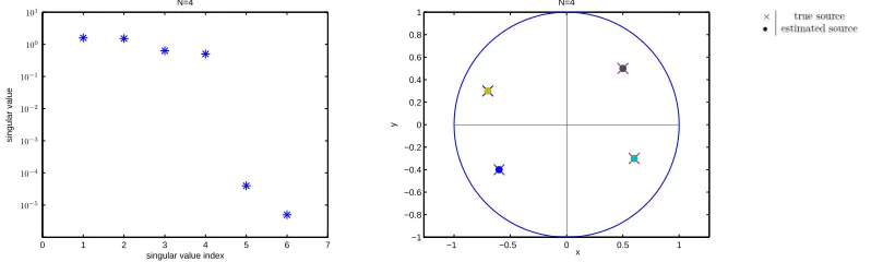
meshing of distributed points on the unit sphere using spherical coordinates. Starting with 252sensors over the
domain’s boundary, we were able to identify the number and 2D location of up to 4 monopoles. Indeed, this is shown in Figure 2 and Figure 3 that presents the singular values for the Hankel matrices HN¯ for the 2Dxy
projection for 4 and 5 monopoles and their corresponding projected positions respectively. We can notice that using the convenient threshold and noting the occurrence of the large gap in the singular value distribution of
HN¯, the number and the precise localization of 4 monopoles can be well-approximated for 252mesh points while
this isn’t the case for more than 5 monopoles. This validates that the accuracy in the monopoles localization and their number identification decrease as the number of monopoles increases which is consistent with the estimate (7).
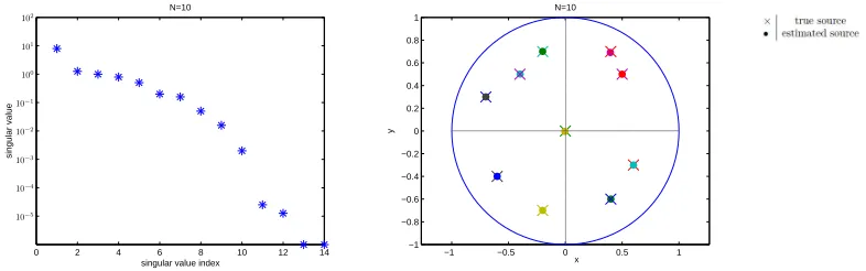
On the other hand, if one possesses more sensors, for instance 502 sensors, the 5 monopoles can be well
approximated as shown in Figure 4. By increasing gradually the number of sensors, we can reconstruct precisely the number and the position up to 10 monopoles. The latter is obtained when using 1002 sensors (see Figure
5). Although, as we have tested, meshing more finely leads also to identify much more than 10 monopoles, a higher number of sensors becomes ”unrealistic”.
0 1 2 3 4 5 6 7
10−5
10−4
10−3
10−2
10−1
100
101
singular value index
singular value
N=4
−1 −0.5 0 0.5 1
−1 −0.8 −0.6 −0.4 −0.2 0 0.2 0.4 0.6 0.8 1
x
y
N=4
0 1 2 3 4 5 6 7
10−5
10−4
10−3
10−2
10−1
100
101
singular value index
singular value
N=5
−1 −0.5 0 0.5 1
−1 −0.8 −0.6 −0.4 −0.2 0 0.2 0.4 0.6 0.8 1 x y N=5
Figure 3. Singular values ofHN¯, ¯N = 6 and the localization results projected on thexyplane for N= 5 with 252 sensors.
0 1 2 3 4 5 6 7 8 9
10−5
10−4
10−3
10−2
10−1
100
101
singular value index
singular value
N=5
−1 −0.5 0 0.5 1
−1 −0.8 −0.6 −0.4 −0.2 0 0.2 0.4 0.6 0.8 1 x y N=5
Figure 4. Singular values ofHN¯, ¯N = 8 and the localization results projected on thexyplane for N= 5 with 502 sensors.
0 2 4 6 8 10 12 14
10−5
10−4
10−3
10−2
10−1
100
101
102
singular value index
singular value
N=10
−1 −0.5 0 0.5 1
−1 −0.8 −0.6 −0.4 −0.2 0 0.2 0.4 0.6 0.8 1 x y N=10
Figure 5. Singular values ofHN¯, ¯N= 14 and the localization results projected on thexyplane for N= 10 with 1002sensors.
As mentioned before, the numerical results can be enhanced using an important number of sensors which isn’t always trivial since the number of sensors is limited. Hence, noting that the projected separability coefficient plays a role in the estimation stability as seen in (7), a good technique to obtain a better estimation is to choose the best projection plane that leads to the highest separability coefficient. Therefore, fixing the number of sensors to 352sensors, the following subsection consists to find the best projection that enables us to recuperate
Remark 3.2. We draw the attention of the reader to the fact that in the case of 352 sensors, the numerical
error can be seen as noise equivalent to 6% perturbation. Thus, according to (7), the separability coefficient still plays a role in the identification of the sources. However, when increasing the number of sensors to 1002
sensors, equivalent to 2% noise, this error is negligible with respect to the separability coefficient. Therefore, the latter wouldn’t have a great influence on the source reconstruction, which justifies the choice of just 352
sensors.
3.2.
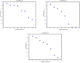
Obtaining the 3D coordinates and the effect of the separability coefficient
To obtain the 3Dcoordinates of the sources, we use consequently the test functions projected on the 2Dplanes as shown in Figure 6 and Figure 7 in the case of 5 monopoles. Note that, theoretically the number of sources must be the same whatever the complex plane onto which the projections are performed (distinct projections). However, numerically the situation may be different since the number depends also on the separability of these projections. This is, also, observed in the stability estimate (7). Therefore, it is preferable to calculate the rank of the three consecutive Hankel matrices corresponding to the test functions v, ¯v, ˜v and then we consider the number of sources as their maximum.
0 1 2 3 4 5 6 7 8 9
10−5
10−4
10−3
10−2
10−1
100
101
singular value index
singular value
N=5 (plane xy)
0 1 2 3 4 5 6 7 8 9
10−5
10−4
10−3
10−2
10−1
100
101
singular value index
singular value
N=5 (plane yz)
0 1 2 3 4 5 6 7 8 9
10−5
10−4
10−3
10−2
10−1
100
101
singular value index
singular value
N=5 (plane xz)
−1 −0.5 0 0.5 1 −1
−0.8 −0.6 −0.4 −0.2 0 0.2 0.4 0.6 0.8 1
x
y
N=5 (plane xy)
−1 −0.5 0 0.5 1
−1 −0.8 −0.6 −0.4 −0.2 0 0.2 0.4 0.6 0.8 1
y
z
N=5 (plane yz)
−1 −0.5 0 0.5 1
−1 −0.8 −0.6 −0.4 −0.2 0 0.2 0.4 0.6 0.8 1
x
z
N=5 (plane xz)
Figure 7. Localization results forN= 5 in thexy,yzandxz planes.
3.3.
Error using Gaussian noise
Reconstruction stability on thexyprojections for 3 monopoles with respect to the noise level is examined in Figure 8. In fact, Gaussian noise is added tof (andg) where the noise standard deviation added varies from 10−4 to 100%. We note that the localization error increases as the percentage of the noise added increases and
the curves show a H¨older form, consistent with the stability estimates (7).
10−4 10−3 10−2 10−1 100
10−3
10−2
10−1
100
Guassian noise %
localization error
N=3
Figure 8. The maximum localization error with respect to the noise level forN= 3.
3.4.
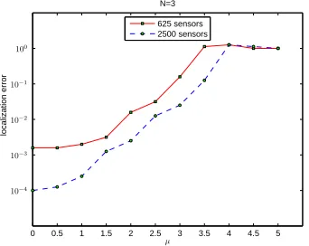
Effect of changing
µ
This is consistent with the stability result (7) and this shows that in practice, taking a small enough absorption coefficient leads to a better estimation. Moreover, this phenomenon with negativeµstands for diffusion rather than propagation that uses positive coefficient µ(corresponding to the wave number). In comparison with the results obtained in [1, 11], we notice that the increase in the negative µ increases the localization error more dramatically and faster. Note that, in Figure 9, we have also presented the effect of the number of sensors on the localization estimation which proves that the finer mesh improves the reconstruction process.
0 0.5 1 1.5 2 2.5 3 3.5 4 4.5 5
10−4
10−3
10−2
10−1
100
µ
localization error
N=3 625 sensors 2500 sensors
Figure 9. The maximum localization error when changingµforN= 3.
References
[1] B. Abdelaziz, A. EL Badia, and A. El Hajj,Reconstruction method for solving some inverse source problems in an elliptic equation from a single Cauchy data, submitted, (2013).
[2] B. Abdelaziz, A. El Badia, and A. El Hajj,Reconstruction of extended sources with small supports in the elliptic equation
∆u+µu=F from a single Cauchy data, Comptes Rendus Mathematique, 351 (2013), pp. 797–801.
[3] C. Alves, R. Kress, and P. Serranho,Iterative and range test methods for an inverse source problem for acoustic waves, Inverse Problems, 25 (2009), pp. 055005, 17.
[4] S. R. Arridge,Optical tomography in medical imaging, Inverse Problems, 15 (1999), pp. R41–R93.
[5] S. R. Arridge, O. Dorn, V. Kolehmainen, M. Schweiger, and A. Zacharopoulos,Parameter and structure reconstruction in optical tomography, in Journal of Physics: Conference Series, vol. 135, IOP Publishing, 2008, p. 012001.
[6] Y.-S. Chung and S.-Y. Chung,Identification of the combination of monopolar and dipolar sources for elliptic equations, Inverse Problems, 25 (2009), pp. 085006, 16.
[7] Y.-S. Chung, J. E. Kim, and S.-Y. Chung,Identification of multipoles via boundary measurements, European J. Appl. Math., 23 (2012), pp. 289–313.
[8] A. El Badia and A. El Hajj, H¨older stability estimates for some inverse pointwise source problems, Comptes Rendus Mathematique, 350 (2012), pp. 1031–1035.
[9] ,Stability estimates for an inverse source problem of Helmholtzs equation from single Cauchy data at a fixed frequency, Inverse Problems, 29 (2013), p. 125008.
[10] A. El Badia and T. Ha-Duong,An inverse source problem in potential analysis, Inverse Problems, 16 (2000), pp. 651–663. [11] A. El Badia and T. Nara,An inverse source problem for Helmholtz’s equation from the Cauchy data with a single wave
number, Inverse Problems, 27 (2011), pp. 105001, 15.
[12] M. Ikehata,Reconstruction of a source domain from the Cauchy data, Inverse Problems, 15 (1999), pp. 637–645.
[13] R. Kress and W. Rundell,Reconstruction of extended sources for the Helmholtz equation, Inverse Problems, 29 (2013), p. 035005.
[14] T. Nara,An algebraic method for identification of dipoles and quadrupoles, Inverse Problems, 24 (2008), pp. 025010, 19. [15] ,Algebraic reconstruction of the general-order poles of a meromorphic function, Inverse Problems, 28 (2012), pp. 025008,
19.
[16] F. Natterer and F. Wubbeling,Mathematical methods in image reconstruction, Society for Industrial and Applied Mathe-matics, Philadelphia, PA, USA, 2001.