N. Champagnat, T. Leli`evre, A. Nouy, Editors
PENALIZATION OF A STOCHASTIC VARIATIONAL INEQUALITY
MODELING AN ELASTO-PLASTIC PROBLEM WITH NOISE
Mathieu Lauri`
ere
1and Laurent Mertz
2Abstract. In a recent work of A. Bensoussan and J. Turi Degenerate Dirichlet Problems Related to the Invariant Measure of Elasto-Plastic Oscillators, AMO, 2008, it has been shown that the solution of a stochastic variational inequality modeling an elasto-plastic oscillator excited by a white noise has a unique invariant probability measure. The latter is useful for engineering in order to evaluate statistics of plastic deformations for large times of a certain type of mechanical structure. However, in terms of mathematics, not much is known about its regularity properties. From then on, an interesting mathematical question is to determine them. Therefore, in order to investigate this question, we introduce in this paper approximate solutions of the stochastic variational inequality by a penalization method. The idea is simple: the inequality is replaced by an equation with a nonlinear additional term depending on a parameter npenalizing the solution whenever it goes beyond a prespecified area. In this context, the dynamics is smoother. In a first part, we show that the penalized process converges towards the original solution of the aforementioned inequality on any finite time interval asngoes to
∞. Then, in a second part, we justify that for eachnit has a unique invariant probability measure. Finally, we provide numerical experiments and we give an empirical convergence rate of the sequence of measures related to the penalized process.
R´esum´e. Dans un travail r´ecent de A. Bensoussan et J. TuriDegenerate Dirichlet Problems Related to the Invariant Measure of Elasto-Plastic Oscillators, AMO, 2008, il a ´et´e montr´e que la solution d’une in´equation variationnelle stochastique mod´elisant un oscillateur ´elasto-plastique excit´e par un bruit blanc admet une unique mesure de probabilit´e invariante. Cette derni`ere est utile en science de l’ing´enieur pour estimer les statistiques des d´eformations plastiques en temps grands d’un certain type de structure m´ecanique. D`es lors, un probl`eme math´ematique int´eressant est de d´eterminer la r´egularit´e de cette mesure. Afin d’´etudier ce probl`eme, nous introduisons ici des solutions approch´ees de l’in´equation par une m´ethode de p´enalisation. Ainsi, l’in´equation est remplac´ee par une ´equation avec un terme nonlin´eaire additionnel d´ependant d’un certain param`etre np´enalisant la solution en dehors d’un domaine admissible. Dans ce contexte, la dynamique stochastique est plus r´eguli`ere. Dans un premier temps, nous montrons la convergence lorsquen tend vers∞du processus p´enalis´e vers la solution de l’in´equation sur tout intervalle de temps fini. Puis dans un second temps, nous montrons que pour chaque n le processus p´enalis´e est dissipatif et qu’il admet une unique mesure invariante. Finalement, nous ´etudions num´eriquement la convergence par rapport au param`etre de p´enalisation et donnons un taux de convergence empirique de la suite des mesures du processus p´enalis´e.
1 Laboratoire Jacques-Louis Lions, Universit´e Paris 7, Paris, France 2 Courant Institute, New York University, New York, New York 10012
c
EDP Sciences, SMAI 2015
1.
Background and Motivations
Phenomena with memory occur naturally in random mechanics. In particular, behaviors of a certain class of mechanical structures, which experience elastic deformations and plastic (permanent) deformations under a random forcing (e.g earthquake), can be represented using an elasto-perfectly-plastic (EPP) oscillator with noise whose dynamics is given (see [F08]) by :
¨
x+c0x˙+F= ˙w, (1.1)
where c0>0 is the viscous damping coefficient, w is a Wiener process and with the initial displacement and
velocity x(0) = 0 and ˙x(0) = 0 respectively. Here F is the nonlinear restoring force depending on a given elasto-plastic boundY >0. This nonlinearity will be explained in subsection 1.1. Recently, A. Bensoussan and J. Turi [BT08] have shown that the dynamics of this oscillator can be described in the mathematical framework of a stochastic variational inequality (SVI). Indeed, denoting (y(t), z(t)) the solution of the following SVI :
(
dy(t) =−(c0y(t) +kz(t)) dt+ dw(t),
(dz(t)−y(t)dt)(φ−z(t))≥0, ∀ |φ| ≤Y, |z(t)| ≤Y, (1.2)
then the velocity of x(t) and the restoring force F can be seen respectively as y(t) and kz(t), here k is a stiffness coefficient. The underlying stochastic process related to this inequality belongs to the class of non-linear and degenerate dynamical systems that constitutes an important research theme in stochastic analysis. In [BT08, BM12], it has been shown that the aforementioned SVI has an appropriate structure for the study in large time of an EPP oscillator in the sense that it allows to show existence and uniqueness of an invariant probability for the solution (see (1.4)). In terms of engineering, this probability measure describes the probabil-ities that (1.1) experiences an elastic or a plastic state for large times, hence it is relevant for pratical purposes. Therefore, a numerical algorithm solving this probability measure has been proposed in [BMPT09] and then it has been applied to the estimation of the frequency of plastic deformation of (1.1) in [FM12].
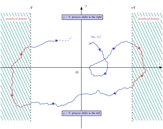
However, from a mathematical point of view, we do not know much about the regularity of this measure. Therefore, in order to investigate this issue, a natural approach in the context of a SVI is to proceed by penalization. The idea consists in replacing the inequality by an equation with an additional nonlinear term. In this way, the solution is not constrained anymore, but when it goes beyond a given prespecified area then the nonlinear term becomes very large such that the solution is “forced” to come back inside that area. In this context, the dynamical system, though still degenerate, is smoother. More precisely, we introduce in the second componentz(t) a penalization term depending on a parameter : n≥1 (for the magnitude of the penalization). Thus we use the notation (yn(t), zn(t)) for this approximate process. The evolution of the system is described by the following stochastic differential equation (SDE) :
dyn(t) =− c0yn(t) +kzn(t)dt+ dw(t), dzn(t) =yn(t)dt−n zn(t)−π(zn(t))
dt
with the initial condition (yn(0), zn(0)) = (y0, z0)
(1.3)
wheren≥1 andπ(z) is the projection ofzonK:= [−Y, Y].
Remark 1.1. Note that the second equation in (1.3)can be written without using explicitly the projection as follows:
The goal of this work, done at CEMRACS2013, is to investigate the properties of solutions of (1.3) that are approximate solutions of (1.2) by a penalization approach. In Theorem 2.1, we prove the convergence of the penalized process toward the solution of the SVI on any finite time interval. Then in Theorem 2.2 , we show that the penalized process has a unique invariant probability measure νn which has a densitymn(y, z). This approximation would be very relevant to understand the properties of the invariant measure related to the SVI.
1.1.
Settings of an elasto-perfectly-plastic oscillator
In the engineering literature, the dynamics of an elasto-perfectly-plastic oscillator is formulated in terms of a stochastic process x(t), which stands for the total deformation of the oscillator that evolves with hysteresis, and whose evolution is described formally by the equation (1.1). The restoring forceFis a nonlinear functional that depends on the entire trajectory{x(s),0≤s≤t}up to time t; its nonlinearity comes from the switching of regimes from a linear phase (called elastic) to a nonlinear one (called plastic), or vice versa. Precisely, the restoring forceFis expressed as follows:
F(t) =
kY, if x(t)−∆(t) =Y,
k(x(t)−∆(t)), if −Y < x(t)−∆(t)< Y, −kY, if x(t)−∆(t) =−Y,
wherekis a stiffness coefficient, ∆(t) is the permanent (or plastic) deformation inx(t) andY is an elasto-plastic bound.
1.2.
Stochastic variational inequality for
(1.1)
From [BT08], we know that the relationship between the velocityy(t) := ˙x(t) andz(t) :=x(t)−∆(t) is governed by a (stochastic) variational inequality as follows : there exists exactly one process (y(t), z(t))∈ R×[−Y, Y] that satisfies the SVI presented in (1.2). A general framework dealing with this class of inequalities can be found in [BL82]. In these settings, the plastic deformation is given by:
∆(t) =
Z t
0
y(s)1{|z(s)|=Y}ds.
Then, it has been shown that there exists a unique limiting probability measure ν for (y(t), z(t)) ast goes to
∞, in the following sense: for all bounded measurable functionsf,
lim
t→∞E[f(y(t), z(t))] =ν(f).
Let us introduce the following notations: D := R×(−Y, Y) is the elastic domain, D+ := (0,∞)× {Y} is the positive plastic domain and D− := (−∞,0)× {−Y} is the negative plastic domain. It is also known from [BT08] that the invariant probability measure ν has support D∪D+∪D− and is characterized by an ultra-weak variational formulation: for all smooth functionsf
Z
D
Af(y, z)ν(dy,dz) +
Z
D+
B+f(y, Y)νY(dy) + Z
D−
-Y +Y
O
× (y0, z0)
penalized domain y >0: process shifts to the right penalized domain
y <0: process shifts to the left
u
u
u u
u
u
u
u
u
u
y
z
Figure 1. We observe (zn(t), yn(t)) : the process is not constrained, but when it goes beyond
a given prespecified area, then the nonlinear term becomes very large so that the solution is “forced” to come back inside that area.
with
Aϕ:=−1
2
∂2ϕ
∂y2 + (c0y+kz)
∂ϕ ∂y −y
∂ϕ ∂z,
B+ϕ:=−
1 2
∂2ϕ
∂y2 + (c0y+kY)
∂ϕ ∂y,
B−ϕ:=− 1 2
∂2ϕ
∂y2 + (c0y−kY)
∂ϕ ∂y.
Moreover, the measureν has a probability density function (pdf)mcomposed of threeL1 functions
(1) an elastic part: m(y, z) onD,
(2) a positive plastic part: m(y, Y) onD+,
(3) a negative plastic part: m(y,−Y) onD−
with the condition m(y, z), m(y, Y), m(y,−Y)≥0 satisfying
Z
D
m(y, z)dydz+
Z
D+
m(y, Y)dy+
Z
D−
2.
Main results
Our first result concerns the convergence of the solution (yn, zn) of (1.3) towards the solution (y, z) of (1.2).
Theorem 2.1. Fix T > 0 and consider the processes (yn(t), zn(t)) and (y(t), z(t)) satisfying (1.3) and (1.2) respectively. Then the following convergence property holds :
lim n→∞E
"
sup t∈[0,T]
n
|yn(t)−y(t)|2+|zn(t)−z(t)|2 o
#
= 0. (2.1)
Moreover, for any λ >0,
lim n→∞E
Z ∞
0
exp(−λt)f(yn(t), zn(t))dt
=E
Z ∞
0
exp(−λt)f(y(t), z(t))dt
. (2.2)
Our second result concerns the existence of an invariant probability for (yn, zn), for fixedn.
Theorem 2.2. The process(yn, zn)admits a unique invariant probability measure, denoted byνn, which admits a densitymn(y, z)with respect to Lebesgue measure. Moreovermn(y, z)must solve (at least in the sense of the distributions) the following Fokker-Planck equation:
∂ ∂z
mn(y, z)[−y+n(z−π(z))]
+ ∂
∂y
mn(y, z)(c0y+kz)
+1 2
∂2
∂y2mn(y, z) = 0, (y, z)∈R 2
. (2.3)
2.1.
Preliminary lemmas and proof of the main results
In this section, we give preliminary lemmas and the proofs of Theorem 2.1 and Theorem 2.2. For the convenience of the reader, the proofs of the preliminary lemmas are given in Section 3.
Let us first present three useful Lemmas for Theorem 2.1. FixT >0.
Lemma 2.3. There existsC(T)>0 such that
∀(m, n)∈(N∗)2, E
" Z T
0
|zm(s)−π(zm(s))||(zn(s)−π(zn(s))|ds #
≤ 1 mnC(T).
Lemma 2.4. The sequence (yn, zn)satisfies the following Cauchy property:
∀ >0, ∃N ∈N, ∀n, m > N, E
"
sup t∈[0,T]
|yn(t)−ym(t)|2+|zn(t)−zm(t)|2 #
< .
Next, we introduce the following notations:
˜
y(t) := lim
n→∞yn(t), z˜(t) := limn→∞zn(t) and ˜
∆(t) := lim n→∞n
zn(t)−π(zn(t)).
Then
Lemma 2.5. The process y˜(t),z˜(t),∆(˜ t)
satisfies the following properties:
(a) y˜(0) = ˜y0, z˜(0) = ˜z0,
(c) |z˜(t)| ≤Y ∀t a.s., and∆˜ satisfies the following properties:
(d) it has bounded variations, (e)
Z t2
t1
1{z˜(t)∈(−Y,Y)}d ˜∆(t) = 0 ∀t1≤t2 a.s., (f) d˜z(t) = ˜y(t)dt −1{z˜(t)=±Y}d ˜∆(t).
We will also formulate the following Theorem from [BL82] (page 49) in our context as follows:
Theorem 2.6 ( [BL82]). There exists a unique process y˜(t),˜z(t),∆(˜ t)
taking values in R2 and satisfying properties (a)− (f). Moreover this solution is characterized by the two following properties:
(i) y,˜ z˜
is continuous, adapted, a.s. for each twe have: |z˜(t)| ≤Y and:
˜
y(t)−y0+ Z t
0
c0y˜(s) +kz˜(s)ds−w(t)
and z˜(t)−z0− Z t
0
˜
y(s)ds
are of bounded variation, and are zero fort= 0. (ii) For any (ϕ1, ϕ2)∈R×[−Y, Y],
ϕ1−y˜(t)
· d˜y(t) + (c0y˜(t) +kz˜(t))ds−dw(t)
+ ϕ2−z˜(t)
· d˜z(t)−y˜(t)dt
≥0.
Lemma 2.3 is employed in the proof of Lemma 2.4 and then Lemmas 2.4, 2.5 and Theorem 2.6 are employed directly in the proof of Theorem 2.1 as shown below.
Proof of Theorem 2.1. First, we proceed with the convergence: by Lemma 2.4, there exists a limit{(˜y(t),˜z(t)), t≥
0} in the sense of the normE
h
supt∈[0,T]
|y˜(t)|2+|z˜(t)|2 i for {(y
n(t), zn(t)), t ≥0} as n goes to ∞. Then,
we identify the limit: by Lemma 2.5, we can apply Theorem 2.6 to ˜y(t),z˜(t)
. Indeed, point (ii) of the characterization given by Theorem 2.6 rewrites:
dy(t) =−(c0y(t) +kz(t))ds+ dw(t)
and ϕ−z(t)
· dz(t)−y(t)dt
≥0, ∀ϕ∈[−Y, Y],
which matches, together with points(a)and(c)of Lemma 2.5, the SVI described by (1.2). Hence ˜y(t),˜z(t)
satisfies the SVI (1.2) and then: y˜(t),z˜(t)
= y(t), z(t)
(by uniqueness of the solution). Finally, as f is bounded, for all >0, there existsT>0 such that
E
Z ∞
0
exp(−λt) f(yn(t), zn(t))−f(y(t), z(t))
dt
=E
" Z T
0
exp(−λt) f(yn(t), zn(t))−f(y(t), z(t))
dt
#
+ 2.
Hence, relying on the above decomposition, it is clear that (2.1) implies (2.2).
Next, we present two useful Lemmas for Theorem 2.2.
Lemma 2.7. Fix n > c0,
∀t >0 Ey2n(t) +kz 2 n(t)
≤ce−c0t+C
n
with c:=y2
0+kz02 andCn:= 2 kn (1−c0
n)
Let us introduce some notations. In the followingCbdenotes the space of continuous and bounded functions on
R, and the operatorPn(t) is defined by: Pn(t)φ(y, z) =E[φ(yn(t), zn(t))|(yn(0), zn(0)) = (y, z)] whereφ∈ Cb. We denote byµn(t) the probability law of (yn(t), zn(t)) on R2,B, whereBis the Borelσ-field onR2, that is:
µn(t)φ:=E[φ yn(t), zn(t))] =µn(0)(Pn(t)φ) forφ∈ Cb.
We also define, forT >0, the probability lawµT
n on R2,B
(which corresponds to the ergodic mean) by:
µT nφ:=
1
T
Z T
0
E[φ yn(t), zn(t))]dt= 1
T
Z T
0
µT
n(0)(Pn(t)φ)dt forφ∈ Cb.
Lemma 2.8. For any sequence Ti↑ ∞, the sequence{µTni}i≥1 is tight.
Lemma 2.7 is used in the proof of Lemma 2.8 which, in turn, is employed directly in the proof of Theorem 2.2 as shown below.
Proof of Theorem 2.2. We will exhibit a tight sequence of measures so that we can extract a subsequence which converges to an invariant measure for (yn, zn). Consider a sequence Ti ↑ ∞. For anyµn(0),
µTi
n is tight by
Lemma 2.8, hence there exists a subsequence nµTnij o
j≥1that converges weakly to a certain measureµn,i.e:
∀φ∈ Cb, µ Tij n (φ)−→
j µn(φ).
Thenµn is invariant since:
µn(Pn(t)φ) = lim j µ
Tij
n (Pn(t)φ)
= lim j
1
Tij Z Tij
0
µn(0) (Pn(s)Pn(t)φ) ds
= lim j
1
Tij Z Tij
0
µn(0) (Pn(s+t)φ) ds
= lim j
1
Tij Z t+Tij
t
µn(0) (Pn(s)φ) ds
= lim j
1
Tij Z Tij
0
µn(0) (Pn(s)φ) ds=µn(φ).
Next, uniqueness of the invariant measure and the existence of a density with respect to the Lebesgue measure are deduced from the convergence ofPn(t) at an exponential rate as shown in (2.6). We follow the lines of [GP13] using “Meyn-Tweedie”-type techniques (see for instance [MT93], [DMT95]).
Step 1 : compact sets are petite.This is a consequence of Theorem 1.1 in [DM10]. Indeed, in our case the system rewrites with the notations of [DM10] fort≥0 :
(
dX1
t =F1(t, Xt1, Xt2)dt+σ(t, Xt1, Xt2)dwt
dX2
t =F2n(t, Xt1, Xt2)dt,
with :
Xt1=yn(t), Xt2=zn(t), σ(t, y, z) = 1,
F1(t, y, z) =F1(y, z) =−(c0y+kz), F2n(t, y, z) =F n
2(y, z) =y−n(z−πn(z)),
where the superscript denotes the dependence ofF2onn, the penalization parameter. Then it is straightforward
to verify that the assumptions of Theorem 1.1 in [DM10] are satisfied. Thus for each measureµT
n, this theorem provides a density estimate (which depends onT) yielding the absolute continuity with respect to the Lebesgue measure. More precisely, we have that for any compactKofR2, there exists a constantαT ,K such that for any
t≤T and (y, z)∈R2:
Pn(t)((y, z),·)≥αT ,Kλ2(·)
whereλ2denotes the Lebesgue measure onR2. From this we deduce directly that compact sets are petite, that is : for every compact setK ofR2, there exist a probability aon R+ and a non-trivialσ-finite measureνa on the Borel sets ofR2such that for every (y, z)∈K, we have :
Z ∞
0
Pn(t)((y, z),·)a(dt)≥νa(·).
Step 2 : drift condition.Define the following real-valued function V on R2: V(y, z) = y2+kz2. We will prove that V is a Lyapunov function and satisfies a certain drift condition; this yields the conclusion thanks to Theorem 2.1 of [DMT95]. Let us denote byAn the infinitesimal generator of the penalized system : for any smooth function φwith compact support inR2:
Anφ(y, z) = 1
2∂yyφ−(c0y+kz)∂yφ+ y−n[z−π(z)]
∂zφ.
Claim 1 : V is a Lyapunov function forAn for any n≥0, in the following sense :
lim sup |(y,z)|→∞
AnV(y, z) =−∞
where|(·,·)|denotes the Euclidean norm onR2. This is true since :
AnV(y, z, t) = 1−(c0y+kz)2y+ y−n[z−π(z)]
2kz= 1−2c0y2−2knz2+ 2knπ(z)z
which tends to−∞as|(y, z)| → ∞, for anyn≥0.
Claim 2 : V satisfies the “drift condition for the extended generator” as defined in [DMT95] : there exists a compact setC of R2 and positive constantsα˜ andβ˜ such that :
AnV ≤β˜−αV˜ on C. (2.5)
Let ˜β= 1 and ˜α <2 min{c0, n}. Then
AnV(y, z)−β˜+ ˜αV(y, z) =−2c0y2−2knz2+ 2knπ(z)z+ ˜α(y2+kz2)
≤(˜α−2c0)y2+ (˜α−2n)kz2+ 2nY k|z|
which tends to−∞since the coefficients ofy2andz2 are negative by definition of ˜α. More precisely, the above
upper bound is non positive as soon as 2nY
2n−α˜ ≤z. Hence, for instance, condition (2.5) holds on the compact set
C:= [0,1]×h 2nY 2n−α˜,
2nY 2n−α˜+ 1
i
Step 3 : exponential convergence.By Steps 1 and 2, we can now apply Theorem 5.2 of Down et al. [DMT95] and obtain the existence of constantsγ1 andγ2 (which may depend onnbut not ont,y andz) such that :
sup {f,|f|≤1}
Pn(t)f(y, z)−µn(f)
≤γ1V(y, z) exp(−γ2t) =γ1 y2+kz2
exp(−γ2t). (2.6)
3.
Proof of Lemmas
Proof of Lemma 2.3. The proof is split into three steps. In the first step, we show that
E
Z T
0
(yn(s))2ds≤C(T), C(T) :=
y2
0+kz20+ 2T
2c0
. (3.1)
Indeed, from (1.3) we deduce by Itˆo’s formula:
(
d y2 n(t)
=−2c0y2n(t)dt−2kyn(t)zn(t)dt+ 2yn(t)dw(t) + 2dt
kd z2 n(t)
= 2kyn(t)zn(t)dt−2knzn2(t)dt+ 2knzn(t)π(zn(t))dt.
Combining these two equations we have:
d y2 n(t)
+kd z2 n(t)
+ 2c0y2n(t)dt= 2knzn(t) π(zn(t))−zn(t)
dt+ 2yn(t)dw(t) + 2dt.
Integrating over [0, t] and considering then the expectation, we have:
Eyn2(t)
+kEzn2(t)
+ 2c0E
Z t
0
y2 n(s)ds
=y2 0+kz
2
0+ 2knE Z t
0
zn(s) π(zn(s))−zn(s)ds
+ 2t
≤y2 0+kz
2 0+ 2t
so that
E
" Z T
0
yn2(s)ds #
≤ y
2
0+kz20+ 2T
2c0
sincex(π(x)−x)≤0 for anyx∈R. Next, in the second step, we show that
Z T
0
(zn(s)−π(zn(s)))2ds≤ 1
n2 Z T
0
(yn(s))2ds (3.2)
Indeed, letϕbe the function defined onRbyϕ(x) := (x−π(x))2. Then:
dϕ(zn(s)) = 2 (zn(s)−π(zn(s))) [yn(s)−n(zn(s)−π(zn(s)))] ds = 2yn(s) [zn(s)−π(zn(s))] ds−2nϕ(zn(s))ds.
Hence, integrating over [0, t] and noticing thatϕ(zn(0)) = 0 (since|zn(0)|=|z|< Y):
ϕ(zn(t)) = 2 Z t
0
yn(s) [zn(s)−π(zn(s))] ds−2n Z t
0
which can be rewritten as:
Z t
0
ϕ(zn(s))ds= 1
n
Z t
0
yn(s) [zn(s)−π(zn(s))] ds− 1
2nϕ(zn(t))
≤ 1 n s Z t 0 y2 n(s)ds
s Z t
0
ϕ(zn(s))ds
yielding (3.2). Finally, we conclude in the last step by using (3.1) and taking the expectation in (3.2) to deduce that
E
Z T
0
(zn(s)−π(zn(s)))2ds≤
C(T)
n2 . (3.3)
Then we apply the Cauchy-Schwarz inequality onER0T(zn(s)−π(zn(s)))(zm(s)−π(zm(s)))dsto get the result.
Proof of Lemma 2.4. Letn, m∈N,by Equation (1.3) for (yn(t), zn(t)) and (ym(t), zm(t)), we have:
(
d(yn(t)−ym(t)) =−
c0(yn(t)−ym(t)) +k(zn(t)−zm(t))
dt
d(zn(t)−zm(t)) = (yn(t)−ym(t))dt−n
zn(t)−π(zn(t))
dt+m
zm(t)−π(zm(t)) dt. Hence: 1 2d
(yn(t)−ym(t))2=−c0(yn(t)−ym(t))2dt−k(yn(t)−ym(t))(zn(t)−zm(t))dt
k
2d
(zn(t)−zm(t))2
=k(yn(t)−ym(t))(zn(t)−zm(t))dt
+k(zn(t)−zm(t))
−n zn(t)−π(zn(t))
+m zm(t)−π(zm(t))
| {z }
Rm,n(t)
dt,
whereRm,n(t) :=−n zn(t)−π(zn(t))
+m zm(t)−π(zm(t))
. Combining these two equations and integrating over [0, t], we have:
1
2(yn(t)−ym(t))
2+k
2(zn(t)−zm(t))
2+c 0
Z t
0
(yn(s)−ym(s))2ds
=k
Z t
0
(zn(s)−zm(s))Rm,n(s)ds
≤(m+n)
Z t
0
zn(s)−π(zn(s))zm(s)−π(zm(s))ds
where we use the following property of the projectionπ(.) : for any two pointsxandx0 in
R,
(x0−x)(x−π(x))≤(x0−π(x0))(x−π(x)).
And we then apply Lemma 2.3 to get
E
"
sup t∈[0,T]
|yn(t)−ym(t)|2+|zn(t)−zm(t)|2 #
≤C(T)
1 m + 1 n .
Proof of Lemma 2.5. Proof of (a)and (b): Notice that ˜y(0),z˜(0)
= (y0, z0) by definition of (˜y,z˜), and (˜y,˜z)
is adapted and continuous a.s., as a consequence of uniform convergence, which stems from Lemma 2.4.
Proof of (c): For each t, we a.s. have |z˜(t)−π(˜z(t))| = 0, i.e. |z˜(t)| ≤ Y. Indeed Equation (3.3) yields successively : E
h P
n RT
0 (zn(s)−π(zn(s)))
2dsi <+∞, hence : P n
RT
0 (zn(s)−π(zn(s)))
2ds <+∞, and thus :
RT
0 (zn(s)−π(zn(s)))
2ds −−→a.e.
n 0. Then, from the converse of Lebesgue’s Theorem, we have that there is a subsequence (nk)k>0 s.t. :
|znk(s)−π(znk(s))| a.e.
−−→
k 0. Finally we have, for this subsequence, that :
|z˜(t)−π(˜z(t))| ≤ |z˜(t)−znk(t)|+|znk(t)−π(znk(t))|+|π(znk(t))−π(˜z(t))| a.e.
−−→
k 0
sincezn(t) converges to ˜z(t). This concludes the proof of (c).
Let us now prove (d), (e) and (f ). We will denote by C(A, B) the set of continuous functions from A
to B (where A and B are metric spaces) and by||k||V T the total variation of a function k : [0, T] →R, i.e. ||k||V T :=
RT
0 d|k|(s). We also remind thatK= [−Y, Y].
Proof of (d): Remark that ˜∆ is the uniform limit of ∆n(t) := Z t
0
yn(s)ds−zn(t) +zn(0) and {∆n, n∈N∗}
is uniformly bounded in total variation. Indeed, recall that we have dzn(t) =yn(t)dt−n
zn(t)−π(zn(t))
dt.
Hence : d∆n(t) =n
zn(t)−π(zn(t))
dt. As a consequence :
||∆n||V T = Z T
0
d|∆n|(t) =n Z T
0
sign(zn(t))
zn(t)−π(zn(t))
dt
≤n√T
s Z T
0
zn(s)−π(zn(s)) 2
ds (by Cauchy-Schwarz inequality)
≤pT C(T) (by (3.3))
which gives a uniform inn. Hence ˜∆ is of bounded variation by the following lemma of [GPP96] (that we state with our notations for simplicity) :
Lemma 3.1 (see Lemma 5.8 of [GPP96]). Let zn ∈ C [0, T],R be a sequence that converges uniformly to a
function z˜. Let∆n ∈ C [0, T],Rbe a sequence that converges uniformly to∆˜ and such that:
a.s. ∃C, ||∆n||V T ≤C.
Then:
a.s. ||∆˜||V T < C
and
Z T
0
znd∆n−−−−→ n→∞
Z T
0
˜
zd ˜∆. (3.4)
This concludes the proof of (d).
Proof of (e): By (3.4), for everyx∈[−Y, Y]:
Z T
0
˜
z(t)−x
Lemma 3.2 (see Lemma 2.1 of [GPP96]). Let z˜ ∈ C [0, T], K
and ∆˜ ∈ C [0, T],R a function of bounded
variation, such that for all x∈K:
Z T
0
˜
z(t)−x
d ˜∆(t)≥0.
Then: Z T
0
1K˚ z˜(t)d ˜∆(t) = 0.
We obtain that :
Z T
0
1(−Y,Y) ˜z(t)
d ˜∆(t) = 0
which yields the result.
Proof of (f ): Letn→ ∞in the second equation of the penalized problem (1.3): dzn(t) =yn(t)dt −n·
zn(t)−π(zn(t))
dt=yn(t)dt −d∆n(t).
In the limit we have: d˜z(t) = ˜y(t)dt −d ˜∆(t).Moreover by (e), d ˜∆(t) =1{z˜(t)=±Y}d ˜∆(t) which concludes the
proof of (f ).
Proof of Lemma 2.7. From (1.3) we deduce by Itˆo’s formula:
d dt y
2 n(t)
=−2c0yn2(t)−2kyn(t)zn(t) + 2yn(t) d
dtW(t) + 2
kd
dt z
2 n(t)
= 2kyn(t)zn(t)−2knz2n(t) + 2knzn(t)π(zn(t)).
Combining these two equations and taking the expectations gives:
d dtE
y2 n(t)
+kd
dtE
z2 n(t)
+ 2c0Eyn2(t)
= 2knE[zn(t)π(zn(t))]−2knEzn2(t)
+ 2.
Hence:
d dtE
y2n(t)
+kd
dtE
zn2(t)
+ 2c0Ey2n(t)
≤knEzn2(t)
+kn
Y
2−2kn
Ez2n(t)
+ 2
for any >0. Taking= 2 1−c0
n
, this inequality becomes:
d dtE
y2
n(t) +kzn2(t)
+ 2c0Ey2n(t) +kzn2(t)
≤Cn.
withCn:= 2(1kn−c0 n)
Y2+ 2. The conclusion follows by Gr¨onwall’s lemma.
Proof of Lemma 2.8. We want to prove that for any >0, there exists a compact setK∈ B such that:
∀i∈N µTi
Fix >0 and let δ:= 1 2
p
C, with C :=c+Cn (wherec andCn are defined in Lemma 2.7). We show that
K:= n
(y, z) :|y|+√k|z| ≤ 1 δ o
is appropriate. Indeed for anyi∈N:
1−µTi
n(1K) = 1−
1
Ti Z Ti
0
E[1K(yn(t), zn(t))] dt
= 1− 1 Ti
Z Ti
0
P[(yn(t), zn(t))∈K] dt
= 1
Ti Z Ti
0
P[(yn(t), zn(t))∈/K] dt
≤ 1 Ti
Z Ti
0
P
|yn(t)|> 1 2δ
+P
√
k|zn(t)|> 1 2δ
dt
≤ 1 Ti
Z Ti
0
4δ2
Eyn(t)2+kzn(t)2dt
≤ (by Lemma 2.7 and the definition ofδ)
4.
Numerical experiments
In this section, we present our numerical tools for dealing with experiments on the invariant measures of (1.3) and their convergence rate (recall that Theorem 2.2 shows that these invariant measures admits a density). First, we present a probabilistic algorithm to simulate the trajectories. Then we give a PDE framework to study (2.2). Finally, we give an empirical rate of convergence.
4.1.
Experiments on the invariant measure using probabilistic simulations
For anyn, from Theorem 2.2 we know that (yn, zn), solution of (1.3), has a unique invariant measure, which admits a density. Based on the above probabilistic algorithm, we can now approximate its density. To do so, we use probabilistic simulations, as explained bellow. In a similar manner to what was done in [BMPT09] and [FM12] to solve (1.2), here the solution (yn(t), zn(t)) of (1.3) has explicit formulae (as far as the differentials are concerned) in each phase: either |zn(t)| ≤ Y, zn(t) > Y or zn(t)<−Y. Note that the goal of this work was to propose a first approach to the computation. Therefore, we neglect the issues that may appear at the interface, when zn(t) is in a neighborhood of{−Y, Y}. Let us mention that a possible direction to tackle this kind of issues would be to use the techniques developped in [GM10]. This will be explored in a future work.
4.1.1. Explicit formulae
For the case|zn(t)| ≤Y, the process (yn(t), zn(t)) behaves like a linear oscillator:
dyn(t) =− c0yn(t) +kzn(t)
dt+ dw(t) dzn(t) =yn(t)dt
Therefore, fort∈[0, t0[ witht0:= inf{s≥0 : |zn(s)|=K}we have :
yn(t) =−
c0
2zn(t) +e −c0t
2
n
−ωzsin(ωt) +y+c0 2z
cos(ωt)o+
Z t
0
e−c20(t−s)cos(ω(t−s))dw(s)
zn(t) =e− c0t
2
zcos(ωt) + 1
ω
y+c0 2z
sin(ωt)
+ 1
ω
Z t
0
e−c20(t−s)sin(ω(t−s))dw(s)
where ω :=
√
|4k−c2 0|
2 . Henceyn(t) (resp. zn(t)) is Gaussian variable of mean ey(t, yn, zn) and variance σ 2 yn(t)
(resp. of meanez(t, yn, zn) and variance σz2n(t)), where:
ey(t, yn, zn) =−
c0
2ez(t, yn, zn) +e −c0t
2
n
−ωzsin(ωt) +y+c0 2z
cos(ωt)o
σ2 yn(t) =
Z t
0
e−c0scos2(ωs)ds−c
2 0
4σ
2 zn(t)−
c0
2ω2e
−c0tsin2(ωt).
and:
ez(t, yn, zn) =e− c0t
2
zcos(ωt) + 1
ω
y+c0 2z
sin(ωt)
σ2 zn(t) =
1
ω2 Z t
0
e−c0ssin2(ωs)ds.
The covariance ofyn(t) andzn(t) is given by:
σyz(t) = 1 2ω
Z t
0
e−c0tsin(2ωs)ds− c0 2ω2
Z t
0
e−c0ssin2(ωs)ds.
For the case|zn(t)|> Y, the process (yn(t), zn(t)) satisfies
dyn(t) =− c0yn(t) +kzn(t)
dt+ dw(t) dzn(t) =yn(t)dt−n zn(t)−Ydt
yn(0) =y , zn(0) =z
Then for anyt0, t1 such that on [t0, t1],zn> Y we have:
yn(t1) =e11(t1−t0)yn(t0) +e12(t1−t0)zn(t0) + Z t1
t0 e11(t
1−s)dw(s) + Z t1
t0 e12(t
1−s)nYds
zn(t1) =e21(t1−t0)yn(t0) +e22(t1−t0)zn(t0) + Z t1
t0 e21(t
1−s)dw(s) + Z t1
t0 e22(t
1−s)nYds
with:
e11(t) := 1
λ−−λ+
(n+λ−)etλ−−(n+λ+)etλ+
e12(t) := 1
λ−−λ+
(n+λ−)(n+λ+) etλ+−etλ−
e21(t) :=etλ−−etλ+
e22(t) := 1
λ−−λ+
where:
λ−:=
−(n+c0)− p
(n+c0)2−4(c0n+k)
2
λ+:=
−(n+c0) + p
(n+c0)2−4(c0n+k)
2
Hence yn(t) (resp. zn(t)) is Gaussian variable of mean e+y(t, yn, zn) and variance σ+y(t)2 (resp. of mean
e+
z(t, yn, zn) and variance σz+(t)
2), where:
e+y(t1, yn, zn) =e11(t1−t0)yn(t0) +e12(t1−t0)zn(t0) + Z t1
t0
e12(t1−s)nY ds
=e11(t
1−t0)yn(t0) +e12(t1−t0)zn(t0) +
nY(n+λ−)(n+λ+)
λ−−λ+
e(t1−t0 )λ+−1
λ+ −
e(t1−t0 )λ+−1 λ−
σ+
y(t1)2=(λ−−λ1 +)2
h(n+λ −)2
2λ−
e2(t1−t0)λ−−1−2(n+λ+)(n+λ−)
λ++λ−
e(t1−t0)(λ++λ−)−1
+(n+λ+)2
2λ+
e2(t1−t0)λ+−1
i and: e+
z(t1, yn, zn) =e21(t1−t0)yn(t0) +e22(t1−t0)zn(t0) + Z t1
t0 e22(t
1−s)nY ds
=e21(t1−t0)yn(t0) +e22(t1−t0)zn(t0) +λ−nY−λ+ · h(n+λ
−)(e(t1−t0 )λ+−1)
λ+ −
(n+λ+)(e(t1−t0 )λ−−1)
λ−
i
σ+
z(t1)2= (λ−−λ1
+)2
h 1 2λ+
e2(t1−t0)λ+−1− 2
λ++λ−
e(t1−t0)(λ++λ−)−1
+ 1 2λ−
e2(t1−t0)λ−−1i
Finally:
σ+
yz(t1) = (λ−−λ1
+)2
(n+λ−)(e(t1−t0 )2λ−−1)
2λ− +
(n+λ+)(e(t1−t0 )2λ+−1)
2λ+
−(n+λ−)(e
(t1−t0 )(λ+ +λ−−1)
λ−+λ+ −
(n+λ+)(e(t1−t0 )(λ+ +λ−)−1)
λ−+λ+
For the casezn(t)<−Y, the process (yn(t), zn(t)) satisfies
dyn(t) =− c0yn(t) +kzn(t)
dt+ dw(t) dzn(t) =yn(t)dt−n zn(t) +Y
dt yn(0) =y , zn(0) =z
Then for anyt0, t1 such that on [t0, t1],zn< Y we have:
yn(t1) =e11(t1−t0)yn(t0) +e12(t1−t0)zn(t0) + Z t1
t0
e11(t1−s)dw(s)− Z t1
t0
e12(t1−s)nYds
zn(t1) =e21(t1−t0)yn(t0) +e22(t1−t0)zn(t0) + Z t1
t0 e21(t
1−s)dw(s)− Z t1
t0 e22(t
with the same notations as above. Hence yn(t) (resp. zn(t)) is Gaussian variable of mean e−y(t, yn, zn) and varianceσ−
y(t)2 (resp. of meane−z(t, yn, zn) and varianceσ−z(t)2), where:
e−y(t1, yn, zn) =e11(t1−t0)yn(t0) +e12(t1−t0)zn(t0) + Z t1
t0 e12(t
1−s)nYds
=e11(t
1−t0)yn(t0) +e12(t1−t0)zn(t0)−nY(nλ+−λ−−λ)(n+λ+)
+
e(t1−t0 )λ+−1
λ+ −
e(t1−t0 )λ+−1 λ−
σ−
y(t1)2= (λ−−λ1 +)2
h(n+λ −)2
2λ−
e2(t1−t0)λ−−1−2(n+λ+)(n+λ−)
λ++λ−
e(t1−t0)(λ++λ−)−1
+(n+λ+)2
2λ+
e2(t1−t0)λ+−1i
and:
e−z(t1, yn, zn) =e21(t1−t0)yn(t0) +e22(t1−t0)zn(t0) + Z t1
t0 e22(t
1−s)nYds
=e21(t
1−t0)yn(t0) +e22(t1−t0)zn(t0)−λ−nY−λ+ · h(n+λ
−)(e(t1−t0 )λ+−1)
λ+ −
(n+λ+)(e(t1−t0 )λ−−1)
λ−
i
σz−(t1)2= (λ−−λ1 +)2
h 1 2λ+
e2(t1−t0)λ+−1− 2
λ++λ−
e(t1−t0)(λ++λ−)−1
+ 1 2λ−
e2(t1−t0)λ−−1i
Finally:
σyz−(t1) = (λ−−λ1
+)2
(n+λ−)(e(t1−t0 )2λ−−1)
2λ− +
(n+λ+)(e(t1−t0 )2λ+−1)
2λ+
−(n+λ−)(e
(t1−t0 )(λ+ +λ−−1)
λ−+λ+ −
(n+λ+)(e(t1−t0 )(λ+ +λ−)−1)
λ−+λ+
4.1.2. Simulation algorithm with an Euler scheme
Based on the previous explicit formulae, we have written a C code to approximate the solution of (1.3). Let
T >0, N ∈Nand (tj)j=0...N be the uniform time grid on the interval [0, T], such that tj=jδtwhereδt:=NT. We set Σ,Σ+, and Σ− ∈ M
2,2(R2) such that:
Σ·ΣT =
σy(δt)2 σyz(δt)
σyz(δt) σz(δt)2
, (Σ+)·(Σ+)T =
σ+
y(δt)2 σyz+(δt)
σ+
yz(δt) σz+(δt)2
, (Σ−)·(Σ−)T =
σ−
y(δt)2 σ−yz(δt)
σ−
yz(δt) σ−z(δt)2
.
Let Gj,mj=0...N,m=1,2be a family of independent Gaussian variablesN(0,1). Gaussian variables are generated using Box-Muller formula and the C function random(). Initialize yδt
0, z0δt
= (y0, z0). The finite difference
scheme for (1.3) is written in the following manner: We defineθδt
j andτjδt forj≥0 recursively by: θ0δt=τ0δt= 0 and:
(
θδt
j+1:= inf
tk> τjδt |zδtt
k|=Y
τδt j+1:= inf
tk > θδtj+1
|zδttk|< Y
• Whentk ∈[τjδt, θδtj+1[ (we have |zδttk|< Y), we set:
yδt tk+1 zδt
tk+1
=
ey(δt, y(tk), z(tk))
ez(δt, y(tk), z(tk))
+ Σ·
Gk,1
Gk,2
.
• Whentk ∈[θδtj+1, τjδt+1[ – ifzδt
tk≥Y, we set:
yδt tk+1 zδt
tk+1
=
e+
y(δt, y(tk), z(tk))
e+
z(δt, y(tk), z(tk))
+ Σ+·
Gk,1
Gk,2
.
– ifzδt
tk≤ −Y, we set:
yδt tk+1 zδt
tk+1
=
e−
y(δt, y(tk), z(tk))
e−
z(δt, y(tk), z(tk))
+ Σ−·
Gk,1
Gk,2
.
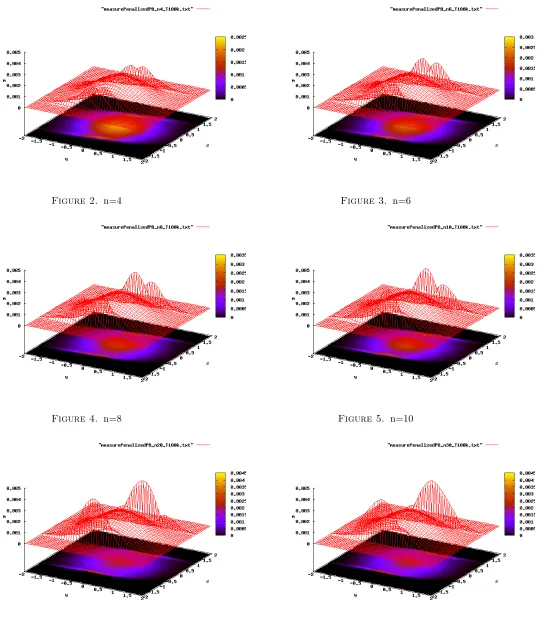
We use the algorithm described above in order to approximate the density of the invariant measure. First, we fix a domainD:= [ymin, ymax]×[zmin, zmax]∈R2and takeNy, Nz∈N∗. This defines a mesh ofNy×Nzpoints with space steps δy := (ymax−ymin)/Ny and δz := (zmax−zmin)/Nz respectively in the y andz directions. Then we simulate the process ytk, ztk
k=0...N and compute, for each cellcof the mesh the number of times it is visited by the process:
{k∈[|0, N|]s.t. ytk, ztk
∈c}
. For the following parameters and lettingnvary, we
obtain Figures 2 to 7:
• ymin =zmin=−5, ymax=zmax= 5,
• Y = 1,
• c0=k= 1,
• T = 100000, δt= 0.001,
• Ny=Nz= 50,
• n= 2,4,6,8,10 according to the figure (see captions).
4.2.
Experiments on the rate of convergence using PDEs
We conjecture the convergence of the invariant measures and we estimate empirically the convergence rate. First, for a bounded measurable functionf,n >0 andλ >0, we consider the functionun
λ(y, z;f) solution of:
λun+Aun =f(y, z) onD
λun+Bn
+un =f(y, z) on ˜D+
λun+Bn
−un =f(y, z) on ˜D−
(Pλ,nf )
Since we assume that both the uniqueness of the invariant measure and the convergence ofλun
λ to it hold (and the simulations presented here tend to show this property), we have thatun
λ(y, z;f) satisfies: ∀(y, z)∈R2,
lim λ→0λu
n
Figure 2. n=4 Figure 3. n=6
Figure 4. n=8 Figure 5. n=10
where: Aϕ:=−1
2ϕyy+ (c0y+kz)ϕy−yϕz, D:=R×(−Y, Y)
Bn +ϕ:=−
1
2ϕyy+ (c0y+kY)ϕy−yϕz+n z−Y
ϕz, D˜+:=R×[Y,+∞[
Bn −ϕ:=−
1
2ϕyy+ (c0y−kY)ϕy−yϕz+n z+Y
ϕz, D˜− :=R×]− ∞,−Y].
Next, define
νn(f) := lim λ→0,λ>0λu
n
λ(y, z;f).
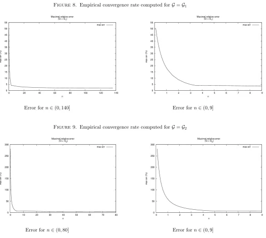
The computation of ν(f) is done using the techniques explained in [BMPT09] (see the Appendix for more details). The error between the measures is computed as follows: given a family G of numerical functions composed of gaussian kernels, we define the maximum relative error:
En(G) := sup ν
n(g)−ν(g)
ν(g) :g∈ G
.
To compute En we assume that there exists a probability densitymn∈L1 satisfying Equation (2.3). For the empirical approximation of this error, we take the following parameters:
• ymin =zmin=−5, ymax=zmax= 5,
• Y = 1,
• c0=k= 1.
To define the families of gaussian functions that we use, we consider the following 9×5 grids (according to axes
y andz respectively), centered on (0,0)
(1) grid 1: with step 0.4 in thez direction and step 1.1 in they direction. (2) grid 2: with step 0.5 in thez direction and step 1.25 in they direction.
Note that the second grid contains nodes on the borders [−L, L]× {−Y}and [−L, L]× {+Y}whereas the first one does not, and that none of the grids contain nodes outside the admissible domainD=R×(−L, L). Then we define G1 (resp. G2) as the family of gaussian functions centered on each node of the first (resp. second)
grid, that is the set of functions gi,ji=1...9,j=1...5defined by:
gi,j(y, z) = exp −(y−yi)2
·exp −(z−zj)2
where (yi, zj) ranges over the nodes ofG1 (resp. G2). The computation of the maximum relative error for the
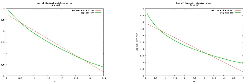
families of test functionsG1 (resp. G2) gives Figure 8 (resp. Figure 9). If we restricts ourselves to the interval
before the error stagnates, we can plot the log of the relative error and see that it is well approximated by a linear function, as in Figure 10. Then the empirical rate of convergence is exponential. More precisely we obtain the following empirical estimation for the convergence rate in each case:
En(G1) = 43.293·exp(−0.740·n) En(G2) = 139.91·exp(−0.728·n).
Acknowledgements
Figure 8. Empirical convergence rate computed forG=G1
Error forn∈(0,140] Error forn∈(0,9]
Figure 9. Empirical convergence rate computed forG=G2
Error forn∈(0,80] Error forn∈(0,9]
like to express their gratitude to Yves Achdou, Alain Bensoussan, St´ephane Menozzi and Olivier Pironneau for their advice and support. Finally, the authors are very grateful to the anonymous reviewer for his detailed and valuable comments that helped us improving the rigor of our work.
Appendix
In this appendix, we explain how to compute the empirical occupation ergodic mean on the spatial mesh,i.e.
Figure 10. Curve fit of the empirical convergence rate
reproduce here the argument for the reader’s convenience. In [BMPT09], a deterministic method alternative to the Monte Carlo method has been developed for solving numerically (1.4). The key point is to solve a stationary PDE with a measurable functionf, satisfying :
Z
D
|f(y, z)|m(y, z)dydz+
Z
D+
|f(y, Y)|m(y, Y)dy+
Z
D−
|f(y,−Y)|m(y,−Y)dy <∞
as right hand side :
λu+Au=f(y, z) inD, λu+B+u=f(y, Y) inD+,
λu+B−u=f(y,−Y) inD−.
Recall from [BMPT09] that this formulation is very significant from a numerical point of view, since it allows to obtain limt→∞E[f(y(t), z(t))] in a way which does not require to solve a time dependent problem. Indeed, it can be shown that ∀(y(0), z(0))∈D, limλ→0λuλ(y(0), z(0)) = limt→∞E[f(y(t), z(t))] and then :
lim
λ→0λuλ(y(0), z(0)) = Z Y
−Y Z +∞
−∞
m(y, z)f(y, z)dydz+
Z +∞
0
m(y, Y)f(y, Y)dy+
Z +∞
0
m(y,−Y)f(y,−Y)dy.
This limit does not depend on (y(0), z(0)).
References
[BL82] A. Bensoussan, J.L. Lions,Impulse Control and Quasi-Variational Inequalities, Dunod, 1982
[BMPT09] A. Bensoussan, L. Mertz, O. Pironneau, J. Turi,An Ultra Weak Finite Element Method as an Alternative to a Monte Carlo Method for anElasto-Plastic Problem with Noise, SIAM J. Numer. Anal.,47(5)(2009), 3374–3396.
[BM12] A. Bensoussan, L. Mertz, An analytic approach to the ergodic theory of stochastic variational inequalities, C. R. Acad. Sci. Paris Ser. I,350(7-8), (2012), 365–370.
[BT08] A. Bensoussan, J. Turi, Degenerate Dirichlet Problems Related to the Invariant Measure of Elasto-Plastic Oscillators, Applied Mathematics and Optimization,58(1)(2008), 1–27.
[DM10] Delarue, F., Menozzi, S.Density Estimates for a Random Noise Propagating through a Chain of Differential Equations. Journal of functional analysis,259-6(2010), 1577–1630.
[F08] C. Feau,Probabilistic response of an elastic perfectly plastic oscillator under Gaussian white noise, Probabilistic Engineering Mechanics,23(1)(2008), 36–44.
[FM12] C. Feau, L. Mertz, An empirical study on plastic deformations of an elasto-plastic problem with noise, Probabilistic Engineering Mechanics,30(2012), 60–69.
[GP13] Gadat, S. and Panloup F.Long time behaviour and stationary regime of memory gradient diffusions. Ann. Inst. H. Poincar´e Probab. Statist., to appear (2013), 1–36.
[GPP96] A. Gegout-Petit, E. Pardoux, Backward stochastic differential equations reflected in a convex domain, Stochastics & Stoch. Rep. 57, no. 1-2 (1996), 111–128.
[GM10] E. Gobet, S. Menozzi.Stopped diffusion processes: overshoots and boundary correction. Stochastic Processes and Their Applications,120-2(2010), 130–162.