www.astesj.com 455
Simulation-Optimisation of a Granularity Controlled Consumer Supply Network Using Genetic
Algorithms
Zeinab Hajiabolhasani *,1,2, Romeo Marian2, John Boland1
1School of Information Technologies and Mathematical Sciences, University of South Australia, 5095, Australia
2School of Engineering, University of South Australia, 5095, Australia
A R T I C L E I N F O A B S T R A C T
Article history:
Received: 29 August, 2018 Accepted: 05 December, 2018 Online: 20 December, 2018
The decision support systems regarding the Supply Chains (SCs) management services can be significantly improved if an effective viable method is utilised. This paper presents a robust simulation optimisation approach (SOA) for the design and analysis of a granularity controlled and complex system known as Consumer Supply Network (CSN) incorporating uncertain demand and capacity. Minimising the total cost of running the network, calculating optimum values of orders and optimum capacity of the inventory associated with each product family are the objectives pursued in this study. A mixed integer non-linear programming (MINLP) model was formulated, mathematically described, simulated and optimised using Genetic Algorithms (GA). Also, the influence of the problem’s attributes (e.g. product classes, consumers, various planning horizons), and controllable parameters of the search algorithm (e.g. size of the population, crossover rate, and mutation rate) as well as the mutual interaction of various dependencies on the quality of the solution was scrutinised using Taguchi method along with regression. The robustness of the proposed SOA was demonstrated by a series of representative case studies. Keywords:
Consumer Supply Network Simulation-Optimisation Granularity
Genetic Algorithms
1. Introduction
The main challenges affecting today’s Supply Chains (SCs) are globalisation, environmental and technological turbulences and rapid changes in economy capacity. They have provoked companies to recognise that, in order to remain competitive in the global market, they need to gain more from their SCs.
Supply Chains are defined as links (relationships) between every unit (enterprise) in a manufacturing process from raw materials to customers. Traditionally, products were made and flowed to consumers through SCs. However, due to globalisation and complexity of the economy, today’s SCs are better characterised as Supply Networks (SNs).
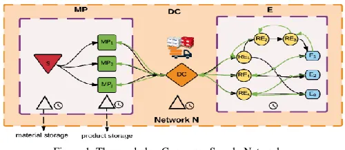
Consumer Supply Networks (CSNs) refer to complex networks consisting of sets of companies working in unison to supply, manufacture, distribute and deliver final products and services to end-users (Figure 1), being controlled by information flow.
CSNs are examples of industrial systems that are naturally large, complex, stochastic, and dynamic. These attributes translate into difficulties in representing the actual behaviour and in
planning, optimising and anticipating performance. Also, the combination of these attributes makes the choice of an appropriate solution methodology difficult at best, if not simply impossible at this point in time [1].
Figure 1 Three echelon Consumer Supply Network
Different methodologies have been utilised to solve this class of complex problem; simulation and optimisation methods are widely used to tackle such problems.
Simulation is a powerful tool for modelling, analysis, and validation of CSNs. However, its major disadvantage is that it will produce a very detailed analysis but strictly for a given
ASTESJ
ISSN: 2415-6698
* Zeinab Hajiabolhasani, Email: [email protected]
www.astesj.com
Special Issue on Multidisciplinary Sciences and Engineering
configuration.Simulation cannot change the configuration of the system, and any optimisation would be searching for the best combination of variables for a given system.
A recurrent, key issue when attempting to optimise CSN is the granularity of the model. An appropriate granularity – the size of the smallest indivisible unit (of product, part, flow, time, etc.) of the process – makes the difference between a successful implementation of the optimisation methodology and an algorithm that does not converge or gets consistently stuck in local optima. Additionally, the choice of the granularity of the model has to be easy to translate in practice – a purely theoretical solution that cannot be implemented in real life is of little help.
This paper is an extension of the work initially has been presented in Intellisys Conference [2] in which a unique simulation optimisation approach (SOA) within an integrated methodology was developed. A small-scale Multi-Period, Multi-Product Consumer Supply Network (MPMPCSN) model, using mixed integer non-linear programming (MINLP) was designed. Then, the optimum quantity of orders was determined incorporating GA optimisation algorithm which simultaneously results in the total inventory cost minimisation. This way, the unique advantages of simulation were incorporated with optimisation method and higher quality solutions were achieved. Also, the quality of the solutions that were obtained by the proposed framework was checked by fine-tuning of the search algorithm’s parameters combining the simulation model with the Taguchi method. Hence, in this study, a series of computational trials on realistic test problems are designed and analysed to demonstrate the generalisability of the proposed SOA for problems of similar size at different granularity levels.
The rest of this article is organised as follows: Section 2 is devoted to reviewing modelling methodologies that were used to solve CSNs problems. Section 3 presents the proposed MINLP model. Section 4 provides details about granularity. The optimisation module of the SOA methodology is described in Section 4. The numerical examples are given in Section 6 and discussed in Section 7. Section 8 concludes the paper.
2. Literature Review
A number of potential solution methods for the class of problems of similar size and complexity have been developed in the literature ranging from classical mathematical programming to hybrid and systematic methods [1, 3].
Optimisation methodologies combined with mathematical models are mainly contributed to solutions validation. A stable optimal solution can be obtained by a given objective function subject to several constraints. However, they are unable to provide the gradient of design space over time [4]. The extent of the optimisation problem cannot be expanded beyond a certain limit as the complexity of the problem adversely affects the computational costs which make less efficient and less practical [5]. This concern can be addressed by using, simulation methodologies.
Simulation models can deal with all attributes of CSNs problems which makes them a powerful analytical tool in this area [6]. In particular, CSN simulation provides a model that suitably represents, processes associated with specific business units such as ordering system, manufacturing plant, distribution centres, etc.
in the presence of uncertainty [7, 8]. Simulation modelling methods alongside with mathematical and models based on algorithms almost always come together. The main advantage of simulation approaches is a possibility to explore what-if scenarios that provide a deeper understanding of the dependencies in a system. The operations of a real system that are usually very dangerous, expensive, or impractical to implement can be evaluated according to their resilience and robustness subject to various predefined inputs (e.g. time horizon, resources, etc.) and at any desired granular level via simulation modelling. Using computer programming, the performance of a real system subject to controlled and environmental changes can be simulated. Therefore, many input values and their combinations can be explored through simulation models [9]. Also, simulation models offer flexibility in developing and assessment of different scenarios, with reasonably high-speed processing. In addition, an embedded standard reporting system make them unique in modelling, analysing, and validating of complex systems.
As pointed out, independent deployment of optimisation and simulation methodologies has some benefits. However, it also has limitations. The main drawback of simulation models is that they can only work with a set configuration of a solution. On the other hand, finding the optimal solution by independently using the traditional optimisation approaches incurs heavy computational cost. Therefore, the integration of the two methods may lead to a uniquely efficient optimisation.
SOA is a key factor of modern design across industries [3]. SOA is often used in the design, modelling and in analyses of systems. It can provide an optimal setting for set of parameters for a simulation model [10]. But due to high computational requirements, scientists have not given much attention to the use of SOA in CSNs [10-12]. Consequently, SOA turns into a hot research topic for optimisation of CSNs. The optimisation core together with a simulation model in SOA, can search the solution space globally (ergodicity of GA) whereas the simulation module acts as a quality assessment unit.
Following the advances in computational power, increased
efforts have been made to leverage simulation for
optimisation/simulation-based optimisation of hybrid systems with behaviours that can be discrete or continuous [13]. CSNs are hybrid systems with a high level of complexity.
Inventory control planning problems have been tackled using many metaheuristic algorithms [5, 14-18]. GA was widely used to solve related problems [19]. Through exploring the solution space, GA finds optimal or near optimal solutions. But, like in other evolutionary algorithms (EA), GA cannot carry out self-validation. GA risks to converge to local optima [20]. Hence, a valid question is whether or not the obtained solution is a high-quality candidate.
statistical methods based on experiments as a more robust approach [22].
In [23], the authors present a multi-echelon SN simulation-based optimisation model for a multi-criteria P-D design. The model offers concurrent optimisation of the network’s structure, the set of the control strategies, and the quantitative parameters of the strategy for control. The modelling, simulation and then optimisation of networked entities are performed using a graphical interface designed in C++ programming. In this study, the candidate solutions are evaluated by a discrete-event simulation (DES) module. A multi-objective GA algorithm is developed aiming at finding compromised solutions regarding structural, qualitative and quantitative variables. The toolbox developed in the research considers a real Production-Distribution model which makes it a unique decision support system. However, there is no evidence shown with regards to parameters tuning of the GA algorithm.
In [24], the authors describe a two-phase Mixed Integer Linear Programming model addressing planning and scheduling systems of a build-to-order SN system. They use GA to optimise the aggregate costs of both subsystems. Three different scenarios were developed, in which distinct recombination rates for genes was used to improve the quality of solutions.
In [25], the researcher model a P-D network over a tactical planning horizon with uncertain demands and capacity. The proposed algorithm incorporates a simulation and an optimisation module; each calculates the total costs of the network for P-D. The problem is mathematically formulated by a MILP, and the fitness function (total cost) is evaluated via the simulation core. Then the solution resulting from the optimisation module is compared with the obtained output from the simulation module recursively. This procedure iterates until there is a set difference between two solutions. This study reports on data obtained from the implementation of the proposed SOA on a SN problem of a reduced scale. Although the simulation and the optimisation modules are both included in the proposed approach, there is no interaction or connection between them. The application of the simulation module is used to produce initial values for the parameters of the mathematical model. Also, the capacity to generalise the model for similar or larger problems was not addressed. Moreover, no evidence was shown around approaching a solution with better quality if different configurations were chosen for the optimisation parameters.
In [15], the authors developed a modified Particle Swarm Optimisation model (MPSO) for a location-allocation Supply Network problem. They formulated a two-echelon Distribution Network (DN) considering multi-product and multi-period inventory, subject to uncertainty of seasonal demands. The determination of the orders quantity and the vendors’ location are pursued as the main objectives in this paper. They use Taguchi to tune the parameters of the MPSO. They considered parameter tuning in their model and they performed a sensitivity analysis for similar problems with different granularity levels.
In a similar study, In [26], the researcher developed a PSO algorithm attempting to find the maximum profit for a channel of a two-echelon SN for a single product. Sales quantity and production rate were used as decision variables of their model. Using a combination of GA, PSO, and simulated annealing (SA), they conduct a detailed sensitivity analysis. However, the
improvement of the proposed heuristic is computed by using another heuristic. This seems very inefficient.
In [27], the authors proposed a simulation optimisation approach to reduce the number of delayed customer orders while costs are kept under control for an integrated production-distribution supply chain. The hybrid modelling combined linear programming and discrete event simulation. This research is a great potential of using SOA approach; however, no effort was made considering the tunning of the control factors of the GA algorithm.
In [28], the researchers developed an agent-based simulation optimisation model through which an online auction policy within the context of the agricultural supply chain was optimised. Three different scenarios namely, oversupply, balance and insufficient supply with different demand and supply quantities were presented to obtain the optimal lot-size and to determine the optimum online auction policy to control inventory. The investigation towards improving the solution quality derived from the proposed methodology was not provided.
An important observation concerning SOA studies is that, in almost all studies, the tuning of the model’s variables (e.g. lead time, production rate, etc.) was only attempted in the optimisation module for small problems. Good examples are included in [20] and [22]. On the other hand, evidence in this regard seems to be missing in some studies [23, 29]. Furthermore, very few ([15, 24]) indicated efforts for tuning the optimisation parameters - selection methodology, mutation, and crossover in GA or swarm’s cognitive and social components in PSO. They reported that this had been done by trial and error - a typical approach used in the majority of OR studies [21]. The simulation model is run several times, then the better solution is selected. Due to the complexity of the interaction of parameters of the search algorithm as well as the high computational cost, it is unclear how many iterations would be sufficient for a given size problem. Besides, as the scale of the problem increases, the complexity of interactions increases exponentially. Therefore, the difficulties corresponding to this class of SNP problems will further escalate if a more detailed model is simulated. So, it is necessary to study in more depth the variation of the solution quality.
This paper presents an integrated simulation-optimisation approach to solve a class of CSN problem using GA. The objective is to minimise the total cost while an optimum/near optimum inventory level associated to each product family is obtained. An important feature of the under-investigated problem is that both demand and the inventory capacity are uncertain. The randomness of the uncertain parameters is captured by the simulation model. The optimal quantities are searched by GA. Also, a fine-tunning mechanism for the optimisation algorithm’s controllable parameters is applied using Taguchi experimental design and ANOVA to improve the quality of the solution. In Section III, the mathematical model, parameters and notations of the proposed problem are summarised.
3. Mathematical Model
The parameters in the model are the following:
𝐷𝑖𝑗𝑡 Demand for product family 𝑖 by retailer 𝑗 in period 𝑡
𝐷𝑖𝑗𝑇 Demand for product family 𝑖 by retailer 𝑗 at the end of
period 𝑇
𝐼0𝑖 Initial inventory level for product family 𝑖
𝑂min𝑖𝑗𝑡 Minimum quantity of product family 𝑖 manufactured for
retailer 𝑗 in period 𝑡
𝑂max𝑖𝑗𝑡 Maximum quantity of product family 𝑖 manufactured for
retailer 𝑗 in period 𝑡
Vmax Maximum capacity of the inventory at DC
𝑉𝑡 Total capacity of inventory at DC in period 𝑡 𝑎𝑖𝑗𝑡 Cost for the ordering of product family 𝑖
𝑏𝑖𝑗𝑡 Cost for purchasing one unit of productfamily 𝑖 at time 𝑡
𝑐𝑖𝑗𝑡 Storage cost for one unit of product family 𝑖 in period 𝑡
𝑑𝑖𝑗𝑡 Handling cost at DC for one unit of productfamily 𝑖 in
period 𝑡
𝑒𝑖𝑗𝑡 Cost for backordering one unit of productfamily 𝑖 in
period 𝑡
𝑓𝑖𝑗𝑡 Cost for transporting one unit of product family 𝑖 in
period 𝑡
𝒜𝑇𝑂 Total cost of ordering at the end of period 𝑇
ℬT𝐼 Total cost of storage in inventory at the end period 𝑇 𝒞T𝐼 Total cost of handling in inventory at the end of period 𝑇 𝒟T𝐷 Total cost of purchasing at the end of period 𝑇
ℰT𝑂 Total costof order shortageat the end period 𝑇
ℱ𝑇𝑂 Total cost of transportation at the end of period 𝑇
𝐶𝑇 The total network costs at the end of period 𝑇
𝜎1 The backorder intensity rate for product family 𝑖 at the
end of period 𝑇
σ2 The capacity severity rate for product family 𝑖 at the end
of period 𝑇
The objective function (1) comprises the minimisation of the total CSN costs, consisting of ordering costs, purchasing costs, transportation costs from manufacturing plants (MP) to retailers (RE), inventory holding and handling costs at the distribution centre (DC), and backordering costs subject to a set of constraints present in (2-4). Constraint (1) represents the quantity of order of a product family 𝑖 in a period 𝑡 bounded by the upper and the lower limits. Note, the maximum quantity of an order for product family 𝑖 from retailer 𝑗 cannot exceed maximum 𝑛 folds of the maximum quantity of the demand for the entire planning period 𝑇. Constrain (2) is the capacity of the inventory denoted by 𝑉𝑇. The order quantity is a positive integer that is normalised between 0 and 1 by (4) denoted by 𝑂́. Table 1 and Table 2 shows a numerical representation of 𝑂𝑖𝑗𝑡, 𝑂𝑖𝑗𝑡́ and 𝐷𝑖𝑗𝑡 for 𝑖 = 3, 𝑗 =5 and 𝑡 = 2.
𝑚𝑖𝑛 ∑ ∑ ∑ 𝐶𝑖𝑗𝑡(𝑂𝑖𝑗𝑡 , 𝐼𝑖𝑗𝑡) 𝑃
𝑖=1 𝑅
𝑗=1 𝑇
𝑡=1
(1)
𝐶𝑇(𝑂𝑖𝑗𝑡, 𝐼𝑖𝑗𝑡) = 𝒜𝑇(𝑂𝑖𝑗𝑡) + ℬ𝑇(𝐼𝑖𝑗𝑡) + 𝒞𝑇(𝐼𝑖𝑗𝑡) + 𝒟𝑇(𝐷𝑖𝑗𝑡) + ℰ𝑇(𝐼𝑖𝑗𝑡) + ℱ𝑇(𝑂𝑖𝑗𝑡) ; ∀ 𝑖, 𝑗 ≥ 0
{
𝒜𝑇(𝑂𝑖𝑗𝑡) = 𝑎𝑖𝑗𝑡. 𝑂𝑖𝑗𝑡 ℬ𝑇(𝐼𝑖𝑗𝑡) = 𝑏𝑖𝑗𝑡. 𝐼𝑖𝑗𝑡 𝒞𝑇(𝐼𝑖𝑗𝑡) = 𝑐𝑖𝑗𝑡. 𝐼𝑖𝑗𝑡
{
𝒟𝑇(𝐷𝑖𝑗𝑡) = 𝑑𝑖𝑗𝑡. 𝐷𝑖𝑗𝑡 ℰ𝑇(𝐼𝑖𝑗𝑡) = 𝑒𝑖𝑗𝑡. 𝐼𝑖𝑗𝑡 ℱ𝑇(𝑂𝑖𝑗𝑡) = 𝑓𝑖𝑗𝑡. 𝑂𝑖𝑗𝑡
𝐶𝑇(𝑂𝑖𝑗𝑡, 𝐼𝑖𝑗𝑡) = 𝑚𝑖𝑛𝑖𝑚𝑖𝑠𝑒 ∑ ∑ ∑ 𝑎𝑖𝑗𝑡. 𝑂𝑖𝑗𝑡+ 𝑃
𝑖=1 𝑅
𝑗=1 𝑇
𝑡=1
𝑏𝑖𝑗𝑡. 𝐼𝑖𝑗𝑡
+ 𝑐𝑖𝑗𝑡. 𝐼𝑖𝑗𝑡+ 𝑑𝑖𝑗𝑡. 𝐷𝑖𝑗𝑡+ 𝑒𝑖𝑗𝑡. 𝐼𝑖𝑗𝑡 + 𝑓𝑖𝑗𝑡. 𝑂𝑖𝑗𝑡
subject to:
𝑂𝑚𝑖𝑛≤ 𝑂𝑖𝑗𝑡≤ 𝑂𝑚𝑎𝑥 (2)
𝑂𝑚𝑖𝑛, 𝑂𝑚𝑎𝑥= [0 𝑛 ∗ max(𝐷𝑖𝑗𝑇)] ; 𝑛 > 1 (3) 𝑉𝑚𝑎𝑥≤ 𝑉𝑇
𝑂𝑖𝑗𝑡= min(⌈𝑂𝑚𝑖𝑛 + (𝑂𝑚𝑎𝑥 − 𝑂𝑚𝑖𝑛 + 1) × 𝑂́⌉ , 𝑂𝑚𝑎𝑥) (4) 0 ≤ 𝑂́ ≤ 1
Numerical representation of 𝑂𝑖𝑗𝑡́ , 𝑂𝑖𝑗𝑡
𝑶́𝒊𝒋𝒕 𝑶́𝟏𝟏𝒕 𝑶́𝟏𝟐𝒕 𝑶́𝟏𝟑𝒕 … 𝑶́𝟏𝒋𝒕
𝑂́21𝑡 𝑂́22𝑡 𝑂́23𝑡 … 𝑂́2𝑗𝑡
⋮ ⋮ ⋮ ⋮ ⋮
𝑂́𝑖1𝑡 𝑂́𝑖2𝑡 𝑂́𝑖3𝑡 … 𝑂́𝑖𝑗𝑡
𝑶́𝒊𝒋𝟏 0.771 0.134 0.681 0.414 0.820
0.699 0.568 0.332 0.247 0.962
0.697 0.425 0.106 0.929 0.581
𝑶́𝒊𝒋𝟐 0.338 0.040 0.182 0.887 0.991
0.670 0.306 0.771 0.135 0.092
0.017 0.394 0.973 0.116 0.447
𝑶𝒊𝒋𝒕 𝑶𝟏𝟏𝒕 𝑶𝟏𝟐𝒕 𝑶𝟏𝟑𝒕 … 𝑶𝟏𝒋𝒕
𝑂21𝑡 𝑂22𝑡 𝑂23𝑡 … 𝑂2𝑗𝑡
⋮ ⋮ ⋮ ⋮ ⋮
𝑂𝑖1𝑡 𝑂𝑖2𝑡 𝑂𝑖3𝑡 … 𝑂𝑖𝑗𝑡
𝑶𝒊𝒋𝟏 161 240 36 111 57
176 172 52 145 231
103 96 97 58 56
𝑶𝒊𝒋𝟐 259 248 53 237 288
212 158 87 124 68
110 99 196 164 132
numerical representation of 𝐷𝑖𝑗𝑡
𝑫𝒊𝒋𝒕 𝑫𝟏𝟏𝒕 𝑫𝟏𝟐𝒕 𝑫𝟏𝟑𝒕 … 𝑫𝟏𝒋𝒕
𝐷21𝑡 𝐷22𝑡 𝐷23𝑡 … 𝐷2𝑗𝑡
⋮ ⋮ ⋮ ⋮ ⋮
𝐷𝑖1𝑡 𝐷𝑖2𝑡 𝐷𝑖3𝑡 … 𝐷𝑖𝑗𝑡
𝑫𝒊𝒋𝟏 259 248 53 237 288
212 158 87 124 68
110 99 196 164 132
𝑫𝒊𝒋𝟐 11 26 17 35 38
72 93 80 42 6
69 61 87 39 85
Note: 𝐷11𝑡 presents the quantity of product family 1 to be manufactured for consumer 1 in time interval 𝑡 = 1 is 259 unit.
The 𝐼𝑖𝑗𝑡 and 𝑂𝑖𝑗𝑡 are related to the decisions regarding the inventory level and the quantity of orders that are calculated by (5). 𝑂𝑖𝑗𝑡 is the main decision variable, since 𝐼𝑖𝑗𝑡 is obtained recursively from 𝑂𝑖𝑗𝑡. The demand quantity, 𝐷𝑖𝑗𝑡, is unknown but bounded. It can be expressed by probabilistic distribution functions such as normal or uniform distribution functions. In this model, a uniform distribution is used to model 𝐷𝑖𝑗𝑡 using (6), where 𝐷𝑚𝑖𝑛, 𝐷𝑚𝑎𝑥 are the lower and upper bounds, respectively.
Also, each product family has a set volume (𝑣𝑖) so the total volume of the order i.e. the total volume occupied by the inventory, 𝑉𝑚𝑎𝑥 , is calculated by (7)
𝐷𝑖𝑗𝑡 ~ 𝑈 (𝐷𝑚𝑖𝑛 , 𝐷𝑚𝑎𝑥) (6)
𝑉𝑚𝑎𝑥= ∑ ∑ ∑ 𝑣𝑖× 𝐼𝑖𝑗𝑡
𝐻
𝑡=1 𝑅
𝑗=1 𝑃
𝑖=1 (7)
𝑣𝑖 ~ 𝑈 (0,1)
If a solution breaks any constraint (𝑐𝑖) it is infeasible and therefore the associated evaluation should be penalised in proportion to how violently they break the constraints. In this problem ∝1 and ∝2 are defined and assigned to the fitness function via (8). The problem size and substantially the changes in the planning period result in changes of ∝1, ∝2.
𝐶𝑇(𝑂𝑖𝑗𝑡, 𝐼𝑖𝑗𝑡) = {(∑ ∑ ∑ 𝒜𝑇. 𝑂𝑖𝑗𝑡+ ℬ𝑇. 𝐼𝑖𝑗𝑡
𝑃
𝑖=1 𝑅
𝑗 𝑇
𝑡=1
+ 𝒞𝑇. 𝐼𝑖𝑗𝑡+ 𝔇𝑇. 𝐷𝑖𝑗𝑡+ ℰ𝑇. 𝐼𝑖𝑗𝑡
+ ℱ𝑇. 𝑂𝑖𝑗𝑡) + 𝛼 𝜎1} × (1 + 𝛽 𝜎2)
(8)
𝜎1=
∑ ∑ ∑ 𝐼𝑇𝑡 𝑅𝑗 𝑃𝑖 𝑖𝑗𝑡
𝑇𝑅𝑃
𝐼𝑖𝑗𝑘< 0
𝜎2=
(𝑉𝑚𝑎𝑥−∑ 𝑉𝑇𝑡 𝑡
𝑉𝑚𝑎𝑥)
𝑇
Also, the average backlogged orders, and the average volume occupied by the inventory are denoted by 𝜎1 and 𝜎2, respectively. In associate with the planning policy in-use, the values of 𝜎1 , 𝜎2 may vary. For example, if the customer satisfaction rate is %100, which means shortages are not allowed and 𝜎1= 0. Conversely, if a company unable to deliver their promises on time then 𝜎1 can be set according to the safety stock level. Note, in both cases, the inventory capacity cannot be exceeded, thus 𝜎2= 0. So, a solution candidate is regarded feasible if both conditions are satisfied.
4. Granularity
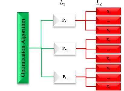
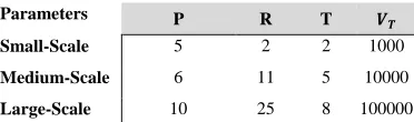
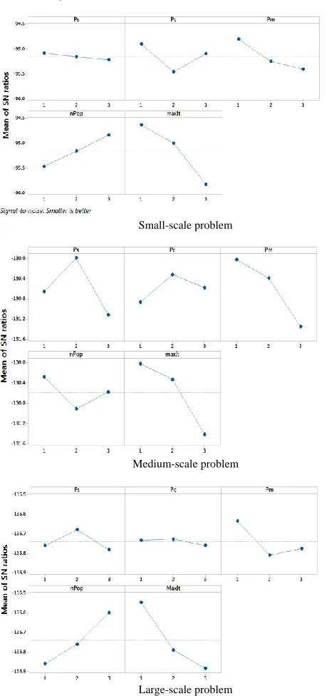
In systems engineering literature, granularity translates into the level of detail one can decide to consider in a model or decision-making process where the same functionality is expressed with different ‘sized’ designs [30]. In SN, the size of the problem determines the granularity level of the problem which has a significant influence on the computation time and the algorithm’s efficiency. Measures such as the number of product families, the number of facilities, planning periods, etc. are some important factors which affect the granularity level [31]. In this study, in order to verify the robustness of the proposed methodology, three case studies with different granularity levels are considered for the design of experiments represented by a tree structure with two levels 𝐿1 and 𝐿2 (Figure 2). The leaves at 𝐿1 denoted by [𝑃𝑆, 𝑃𝑀, 𝑃𝐿], correspond to an individual scenario with a distinct problem size, known as Small, Medium and Large-scale problems. 𝐿1 is developed based on the problem size categories proposed by Mousavi, Bahreininejad, Musa and Yusof [15], shown in Table 3. The roots at 𝐿2 are the number of experiments considered for each category. This is determined according to the number of parameters and the levels of variation of a specific parameter which will be developed using Taguchi method (see Section 6).
𝐿1 𝐿2
Figure 2 Hierarchical structure proposed for implementation phase
Sizes of the proposed instances [15]
Problem Size Product Family (𝑷)
Manufacturing Plants (𝑴𝑷)
Retailer (𝑹𝑬)
Periods (𝑻)
Small [1-5] [1-5] [5-10] [1-3]
Medium [6-10] [1-10] [11-20] [1-5]
Large [11-15] [11-15] [20-30] [6-10]
Note: a problem with 𝑃 = 7, 𝑀𝑃 = 6, 𝑅𝐸 = 11 and 𝑇 = 2 is counted as a Medium-scale problem.
5. Solution Approach
To solve the MPMPCSN problem discussed in this paper, GA optimisation method is used. GA are based on principles of natural selection and genetics to evolve better solutions through multiple consecutive generations. Selection, Crossover and Mutation are implementations in GA of similar phenomena occurring in the natural world. [23]. Based on the quality of solutions, they have a probability to be selected and evolve in new generations and converge towards optimality. Finally, the solutions are tested against termination criteria (evolving procedure). A good search space and genetic operators must maintain an equilibrium between exploration and exploitation and this is key in reaching optimality [32-34]
5.1. Generation and Initialisation
The first step in implementing the GA is to generate a random population of solutions (chromosomes). Chromosomes are resizable according to problem’s attributes and vary based on the problem type, level of complexity, number and type of variables, granularity, etc. Each chromosome consists of several atomic structures - genes representing the characteristics of the solution (e.g. number of suppliers, position of manufacturing plants, types of products considered, etc.) [35]. Real coding has been used for this type of problem (Figure 3).
Figure 3 Chromosome representation
The performance of the GA is affected by two opposing factors; population size and computation time. The larger the population size; the longer takes the computation time. The population size should be large enough to incorporate sufficient variation in one generation from which the children in the next
Op
ti
m
isa
ti
on
A
lgo
rithm
PS
X1
...
Xn
PM
X1
...
Xn
PL
X1
...
Xn
1 𝑂́𝑖𝑗𝑡 𝑂́11𝑡 𝑂́12𝑡 𝑂́13𝑡 … 𝑂́1𝑗𝑡 𝑇𝐶1𝑡
2 𝑂́21𝑡 𝑂́22𝑡 𝑂́23𝑡 … 𝑂́2𝑗𝑡 𝑇𝐶2𝑡
⋮ ⋮ ⋮ ⋮ ⋮ ⋮ ⋮
generations are produced. GA is designed to evolve over a number of generations. Hence, having a large population has a serious impact on the computation time. A carefully selected population size that offers sufficient variety but does permit a fast-enough evolution is needed.
5.2. Genetic Operators: Selection, Crossover, and Mutation Genetic operators may affect the optimal fitness value for the designed algorithm. The GA operators presented in this paper are selection, crossover and mutation. Roulette Wheel, Tournament and Ranked are the most popular selection mechanisms that are used in this study [33, 36].
In the following step, the offspring population is created by applying single point crossover and mutation. So, new offsprings are produced by combining the characteristics of two parents that can be better than both parents if they take the best characteristics from each of the parents. This mechanism should be performed with a certain probability. Throughout this study, 𝑃𝑐 and 𝑃𝑚 are refferring to crossover and mutation probabilities respectively. Two individuals are produced per randomly selected parents followed by mutating gens of offspring population with specified probability. The mutation is implemented to preserve the variety of the solution pool and prevent GA getting stuck in local optima by exploring the entire search space and maintaining diversity in the population [37]. It is likely that some randomly lost genetic information recovered through mutation. Pm should be set carefully
too as such the diversity in the population is preserved but does not negatively affect the overall, fitness of the current population by removing good solutions. Mutation can finely tune the balance between exploration and exploitation. Typically, the mutation rate is small (<2-5%).
5.3. Simulation
After initialising the first population, each chromosome is evaluated for fitness. Fitness function is a metric used to measure the quality of the represented solution. The fitness value of a chromosome is the most important factor in GA evaluation that is always problem dependent [38]. The fitness function defined for MPMPCSN is the minimum cost of running the network. So the lower the fitness value, the higher is the survival chance of a chromosome.
5.4. Stopping Conditions
The optimal/near optimal solution is achieved through an iterative procedure until the stopping condition is satisfied. Choosing the termination criteria depends on the complexity of the problem structure as well as the size of the solution pool [39]. Often, the maximum number of generation is adopted which is the case in this study.
The traditional GA has several shortcomings. As a result of premature convergence, the search parameters (selection, crossover, mutation) may not be very useful towards the end of a search procedure [40]. Also, obtaining an absolute global optimum is not guaranteed, however providing good solutions within a reasonable time is generally expected [41, 42]. Also, GA may not be effective if the starting point in search space was at a great distance from optimal solutions [43]. This deficiency limits the use of GA in real-time applications. However, it can be overcome if GA is hybridised with other local search methods where a closed-form expression of the objective function can be appropriately
performed [42]. Simulation tools are unique methods that are tightly integrated with mathematical and algorithmic based models. Overall, to improve GA performance and obtain accurate solutions, the population size, selection mechanism, crossover and mutation rates and the computational time are required to be turned. Further validation and evaluation of the proposed model and the solution approach is discussed in the following section.
6. Computational Experiments
This section provides experimental results obtained from applying the proposed SOA methodology on practical tests associated to MPMPCSN problems with different granularity levels.
A manufacturing CSN with a central distribution centre is considered in which orders received from consumers are being processed. The demand quantities for 𝑃𝑆, 𝑃𝑀 and 𝑃𝐿 were randomly generated first and remained unchanged throughout the rest of the optimisation algorithm (see. Appendix A, Table 22-Table 24), because the variation of 𝐷𝑖𝑗𝑡 causes changes of other parameters. Also, associated purchase cost per unit of product family 𝑃𝑖 and the corresponding volume 𝑣𝑖 for 𝑃𝑆, 𝑃𝑀 and 𝑃𝐿are given in Appendix A (Table 21). All other related costs of running the network consist of ordering cost, backordering cost, holding cost, handling cost and transportation cost are computed via (9)-(14). In addition, the fixed parameters of the model are presented in Table 4.
𝑎𝑖𝑗𝑡= 0.1 × 𝑑𝑖𝑗𝑡 (9)
𝑏𝑖𝑗𝑡= 0.05 × 𝑑𝑖𝑗𝑡 (10)
𝑐𝑖𝑗𝑡= 0.05 × 𝑑𝑖𝑗𝑡 (11)
1 ≤ 𝑑𝑖𝑗𝑡 ≤ 100 (12)
𝑒𝑖𝑗𝑡= 0.05 × 𝑑𝑖𝑗𝑡 (13)
𝑓𝑖𝑗𝑡= 0.05 × 𝑑𝑖𝑗𝑡 (14)
fixed parameters of the model
Parameters P R T 𝑽
𝑻
Small-Scale 5 2 2 1000
Medium-Scale 6 11 5 10000
Large-Scale 10 25 8 100000
Note: P, R, and T are referred to the Product family, Retailer and Planning period respectively.
7. Results and Discussion
As discussed above, the performance of the GA optimisation algorithm is mostly influenced by its controllable parameters. These parameters are selection method (𝑃𝑠), crossover and mutation rate (𝑃𝑐, 𝑃𝑚), population size (𝑛𝑃𝑜𝑝) and the maximum number of iteration (𝑀𝑎𝑥𝐼𝑡). Thus, though utilising Taguchi Orthogonal Array Design along with Regression Analysis and Optimisation Solver the optimal parameter set was determined. More details are given in the following sections.
7.1. Process of Experiment Design
numbers known as orthogonal arrays. These tables are then used first to reduce the number of experiments, next to determine the most critical parameters with high impact on the outcomes. In this study, we consider the GA controllable parameters as significant factors in 3 levels (Table 7). The Taguchi Orthogonal Array Design (𝐿27 − 35) shown in Table 6 is proposed and created by Minitab.
The 𝐺𝐴 parameters’ level
Granularity Level Small-scale Medium-Scale Large-Scale
Parameters Level 1 Level 2 Level 3
𝑷𝐬 𝑅𝑊 𝑇 𝑅
𝑷𝒄 0.9 0.85 0.8
𝑷𝒎 0.1 0.05 0.025
𝒏𝑷𝒐𝒑 [30 60 120] [100 150 200] [100 200 300]
𝑴𝒂𝒙𝑰𝒕 [200 100 50] [500 400 300] [3500 3000 2000]
𝑅𝑊, 𝑇 and 𝑅 referred to Roulette Wheel, Tournament and Ranked Selection method respectively
The layout of the orthogonal array for 5 factors in 3 levels
No. 𝑷𝒔 𝑷𝒄 𝑷𝒎 𝒏𝑷𝒐𝒑𝑴𝒂𝒙𝑰𝒕
S1 1 1 1 1 1
S2 1 1 1 1 2
S3 1 1 1 1 3
S4 1 2 2 2 1
S5 1 2 2 2 2
S6 1 2 2 2 3
S7 1 3 3 3 1
S8 1 3 3 3 2
S9 1 3 3 3 3
S10 2 1 2 3 1
S11 2 1 2 3 2
S12 2 1 2 3 3
S13 2 2 3 1 1
S14 2 2 3 1 2
S15 2 2 3 1 3
S16 2 3 1 2 1
S17 2 3 1 2 2
S18 2 3 1 2 3
S19 3 1 3 2 1
S20 3 1 3 2 2
S21 3 1 3 2 3
S22 3 2 1 3 1
S23 3 2 1 3 2
S24 3 2 1 3 3
S25 3 3 2 1 1
S26 3 3 2 1 2
S27 3 3 2 1 3
7.2. Signal-to-Noise (S/N) Ratio Method
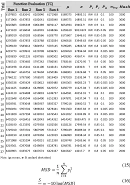
S/N ratios evaluate the size of the apparent effect (signal) against the size of random fluctuations (noise) witnessed in the data. The higher this indicator, the better the compromise is which can be calculated in different ways according to the optimisation problem (minimisation/maximisation) [44]. In this study, S/N ratio values are calculated to determine the best combination of GA control factors. The proposed optimisation algorithm was run four times for each parameter set to obtain more refined solutions. The numerical results for the Small, Medium and Large-scale problem are reported in Table 7, Table 8 and Table 9, respectively.
This problem is aimed to minimise the response value (y). Therefore, to minimise the mean-square deviation (MSD) from the target value 0 and maximise the S/N ratio, MSD has to be
calculated using (15). The signal to noise (S/N) ratio, in this case, is defined by (16), where 𝑛 is the sample size.
Taguchi experimental design and design data of 𝐺𝐴 for small-scale problem
Tri
al
No.
Function Evaluation (TC)
𝝁 𝝈 𝑷𝒔 𝑷𝒄 𝑷𝒎 𝒏𝑷𝒐𝒑 𝑴𝒂𝒙𝑰𝒕
Run 1 Run 2 Run 3 Run 4
1 52545.31 52838.97 52824.62 52798.99 52751.97 138.76 RW 0.9 0.1 30 200 2 57736.13 57984.64 54800.67 56440.22 56740.41 1459.71 RW 0.9 0.1 30 100 3 55082.79 54767.13 55334.41 55983.30 55291.91 516.06 RW 0.9 0.1 30 50 4 57348.28 56895.83 58086.99 58118.95 57612.51 595.84 RW 0.85 0.05 60 200 5 59594.91 58612.27 61314.77 61253.54 60193.87 1321.56 RW 0.85 0.05 60 100 6 60380.16 62646.26 60710.87 59366.54 60775.96 1371.79 RW 0.85 0.05 60 50 7 55536.78 54608.65 55060.74 54506.04 54928.05 471.97 RW 0.8 0.025 120 200 8 55135.85 54540.19 54946.94 56517.07 55285.01 858.15 RW 0.8 0.025 120 100 9 57518.01 59179.99 56537.55 57925.29 57790.21 1094.37 RW 0.8 0.025 120 50 10 52410.97 52718.79 52428.90 52416.20 52493.72 150.24 T 0.9 0.05 120 200 11 53368.53 52881.84 53767.00 52857.57 53218.73 434.73 T 0.9 0.05 120 100 12 58698.26 55432.41 56344.90 57940.46 57104.01 1484.56 T 0.9 0.05 120 50 13 54263.36 56283.66 55064.54 55837.51 55362.27 889.02 T 0.85 0.025 30 200 14 56139.17 56388.68 57656.13 56204.80 56597.20 713.81 T 0.85 0.025 30 100 15 62448.49 94741.69 60631.15 98432.34 79063.42 20304.09 T 0.85 0.025 30 50
16 52413.82 52417.87 52439.46 52418.27 52422.36 11.58 T 0.8 0.1 60 200
17 53546.80 54432.52 53665.56 52804.39 53612.32 666.48 T 0.8 0.1 60 100 18 62686.18 56408.68 56602.45 56552.31 58062.41 3083.61 T 0.8 0.1 60 50 19 54034.56 53650.51 53214.02 53760.76 53664.96 341.24 R 0.9 0.025 60 200 20 56947.05 58519.69 57332.37 56946.45 57436.39 744.73 R 0.9 0.025 60 100 21 62368.65 58889.81 64213.45 64114.90 62396.70 2486.75 R 0.9 0.025 60 50 22 52472.93 52454.69 52466.57 52462.89 52464.27 7.61 R 0.85 0.1 120 200 23 54151.02 54381.73 54913.21 54443.82 54472.45 319.71 R 0.85 0.1 120 100 24 59054.53 58677.67 59390.45 59848.09 59242.69 497.66 R 0.85 0.1 120 50 25 54123.74 53139.69 53600.31 53588.71 53613.11 402.34 R 0.8 0.05 30 200 26 62582.39 57133.15 57636.73 58226.32 58894.65 2498.75 R 0.8 0.05 30 100 27 76782.74 63219.40 67855.77 65419.86 68319.44 5951.48 R 0.8 0.05 30 50
Note: (𝝁: m ean , 𝝈: St andard deviation)
Taguchi experimental design and design data of 𝐺𝐴 for medium-scale problem
Tri
al
No.
Function Evaluation (TC)
𝝁 𝝈 𝑷𝒔 𝑷𝒄 𝑷𝒎 𝒏𝑷𝒐𝒑 𝑴𝒂𝒙𝑰𝒕
Run 1 Run 2 Run 3 Run 4
1 3055303 3053526 3046047 3050184 3051265.00 4074.87 RW 0.9 0.1 200 500 2 3149794 3154852 3180213 3164676 3162383.75 13396.09 RW 0.9 0.1 200 400 3 3372901 3350114 3335613 3323874 3345625.50 21114.59 RW 0.9 0.1 200 300 4 3200575 3185842 3197118 3191536 3193767.75 6464.29 RW 0.85 0.05 150 500 5 3355893 3308538 3369709 3382514 3354163.50 32301.14 RW 0.85 0.05 150 400 6 3499418 3511169 3529597 3529401 3517396.25 14775.75 RW 0.85 0.05 150 300 7 3432256 3440475 3410509 3433997 3429309.25 13022.82 RW 0.8 0.025 100 500 8 3575145 3520148 3586398 3537586 3554819.25 31141.79 RW 0.8 0.025 100 400 9 4555883 4146796 3846552 4203898 4188282.25 290903.67 RW 0.8 0.025 100 300 10 3051447 3066724 3034552 3045986 3049677.25 13368.15 T 0.9 0.05 100 500 11 3156857 3217344 3129544 3179152 3170724.25 37114.87 T 0.9 0.05 100 400 12 3281164 3310920 3406627 3340245 3334739.00 53652.67 T 0.9 0.05 100 300 13 3077422 3072374 3047223 3078703 3068930.50 14727.31 T 0.85 0.025 200 500 14 3182456 3188477 3166677 3221685 3189823.75 23144.54 T 0.85 0.025 200 400 15 3436084 3441521 3417875 3435688 3432792.00 10294.60 T 0.85 0.025 200 300 16 2991777 2972519 2986549 2982617 2983365.50 8146.47 T 0.8 0.1 150 500 17 3057430 3030744 3064818 3033992 3046746.00 16926.05 T 0.8 0.1 150 400 18 3172227 3184862 3188181 3173263 3179633.25 8079.53 T 0.8 0.1 150 300 19 3360788 3373308 3403272 3440016 3394346.00 35280.59 R 0.9 0.025 150 500 20 3503662 3492818 3501245 3457735 3488865.00 21267.49 R 0.9 0.025 150 400 21 6083231 6707308 6357912 5970323 6279693.50 328268.14 R 0.9 0.025 150 300 22 3099402 3117656 3130297 3111689 3114761.00 12846.33 R 0.85 0.1 100 500 23 3243754 3249067 3272814 3255208 3255210.75 12634.31 R 0.85 0.1 100 400 24 3410574 3462829 3421737 3409948 3426272.00 24965.85 R 0.85 0.1 100 300 25 3232477 3281042 3288839 3245727 3262021.25 27198.93 R 0.8 0.05 200 500 26 3372780 3354390 3375793 3360978 3365985.25 10031.33 R 0.8 0.05 200 400 27 3542951 3526380 3567064 3540808 3544300.75 16865.55 R 0.8 0.05 200 300
Taguchi experimental design and design data of 𝐺𝐴 for large-scale problem
Tri
al
No.
Function Evaluation (TC)
𝝁 𝝈 𝑷𝒔 𝑷𝒄 𝑷𝒎 𝒏𝑷𝒐𝒑 𝑴𝒂𝒙𝑰𝒕
Run 1 Run 2 Run 3 Run 4
1 6197853 6182641 6205040 6171968 6189375 14895.51 RW 0.9 0.1 100 3500 2 6171968 6197853 6182641 6205040 6189375 14895.51 RW 0.9 0.1 100 3000
3 6026883 6036349 6064389 6092117 6054934 29462.9 RW 0.9 0.1 100 2000
4 6171329 6156044 6162801 6148266 6159610 9813.874 RW 0.85 0.05 200 3500 5 6189910 6160183 6168566 6183770 6175607 13646.61 RW 0.85 0.05 200 3000 6 6276588 6197853 6256788 6232034 6240816 33949.63 RW 0.85 0.05 200 2000 7 5609430 5583614 5604952 5587145 5596285 12806.33 RW 0.8 0.025 300 3500 8 6219773 6220941 6220798 6296291 6239450 37896.94 RW 0.8 0.025 300 3000 9 6393839 6421235 6397965 6500502 6428385 49567.4 RW 0.8 0.025 300 2000 10 5765313 5783485 5797242 5786545 5783146 13270.95 T 0.9 0.05 300 3500 11 6145198 6115210 6141100 6146131 6136910 14630.8 T 0.9 0.05 300 3000 12 6181667 6166755 6174604 6150186 6168303 13526.68 T 0.9 0.05 300 2000 13 5766122 5797580 5768570 5819409 5787920 25393.04 T 0.85 0.025 100 3500 14 6330538 6295429 6350012 6405480 6345365 46003.23 T 0.85 0.025 100 3000 15 6421425 6446814 6429805 6425072 6430779 11227.04 T 0.85 0.025 100 2000 16 6124129 6234488 6150018 6149727 6164591 48152.91 T 0.8 0.1 200 3500 17 6132648 6141044 6166400 6151393 6147871 14537.94 T 0.8 0.1 200 3000 18 5803931 5783648 5803967 5805327 5799218 10400.52 T 0.8 0.1 200 2000 19 5930494 5953702 5898563 5878441 5915300 33387.83 R 0.9 0.025 200 3500 20 6231820 6227294 6232032 6276543 6241922 23183.89 R 0.9 0.025 200 3000 21 6401559 6416416 6425043 6414352 6414342 9699.475 R 0.9 0.025 200 2000 22 6103190 6123392 6079358 6102566 6102126 17999.54 R 0.85 0.1 300 3500 23 5729010 5873701 5867909 5715137 5796439 86089.04 R 0.85 0.1 300 3000 24 6103190 6123392 6079358 6122019 6106989 20598.34 R 0.85 0.1 300 2000 25 6271088 6235294 6240251 6212358 6239748 24169.66 R 0.8 0.05 100 3500 26 6219361 6297088 6249893 6228781 6248781 34642.66 R 0.8 0.05 100 3000 27 6402903 6433575 6407674 6422437 6416647 14017.7 R 0.8 0.05 100 2000
Note: (𝝁: m ean , 𝝈: St andard deviation)
𝑀𝑆𝐷 =1 𝑛 ∑ 𝑦𝑖
2 𝑛
𝑖=1
(15)
𝑆
𝑁= −10 log(𝑀𝑆𝐷)
(16)
The example of the calculation of S/N ratio for the control parameter 𝑃𝑠 is shown below (column 1 of Table 10) and the results correspond to each case study are summarised in Table 10, Table 11 and Table 12. The difference between the levels of factors in the Table 10- Table 12 determines which parameter has more effect on the quality characteristics (the total cost of the network).
𝐿𝑒𝑣𝑒𝑙 1 =(−94.44 − 95.08 − 94.85 − 95.21 − 95.59 − 95.68 − 94.80 − 94.85 − 94.24)
9 = −95.08
𝐿𝑒𝑣𝑒𝑙 2 =(−94.40 − 94.52 − 95.13 − 94.86 − 95.05 − 98.16 − 94.39 − 94.58 − 95.28)
9 = −95.16
𝐿𝑒𝑣𝑒𝑙 3 =(−94.60 − 95.18 − 95.91 − 94.40 − 94. 𝑡ℎ𝑒 72 − 95.45 − 94.59 − 95.41 − 96.72)
9 = −95.22
𝐷𝑖𝑓𝑓𝑒𝑟𝑒𝑛𝑐𝑒 = | ℎ𝑖𝑔ℎ𝑒𝑠𝑡 𝑣𝑎𝑙𝑢𝑒 | − | 𝑙𝑜𝑤𝑒𝑠𝑡 𝑣𝑎𝑙𝑢𝑒 |
= | −95.22 | − | −95.08 | = 0.14
As it can be seen from Table 10, the control factor 𝑀𝑎𝑥𝐼𝑡, by far is the most important factor that impacts on S/N ratio (1.19), 𝑛𝑃𝑜𝑝 , 𝑃𝑚 , 𝑃𝑐 and 𝑃𝑠 are also significant factors. Table 11 shows 𝑀𝑎𝑥𝐼𝑡, 𝑃𝑠 and 𝑃𝑚 are approximately double of 𝑃𝑐 and 𝑛𝑃𝑜𝑝. Also, in Table 12 while control factor 𝑃𝑐 has a negligible effect in influencing the S/N ratio in 𝑃𝐿 problem, the contribution of all other four parameters (𝑃𝑠, 𝑃𝑚, 𝑛𝑃𝑜𝑝 and 𝑀𝑎𝑥𝐼𝑡) to the S/N is more than 10%.
The S/N ratios computed for the data set 𝑃𝑠, 𝑃𝑐, 𝑃𝑚, 𝑛𝑃𝑜𝑝 and 𝑀𝑎𝑥𝐼𝑡 (Table 10-Table 12) are essential for sketching the S/N
ratio response diagrams for 𝑃𝑆, 𝑃𝑀 and 𝑃𝐿 problems (0). So, a higher S/N ratio is related to a data set with the minimum variation which is considered as the best data set.
The response table of S/N ratio of 𝑃𝑆 Problem
Selection (𝑷𝒔)
Crossover Rate (𝑷𝒄)
Mutation Rate (𝑷𝒎)
Population Size
(𝒏𝑷𝒐𝒑)
Generation (𝑴𝒂𝒙𝑰𝒕)
Level 1 -95.08 -94.90 -94.80 -95.46 -94.63
Level 2 -95.16 -95.46 -95.25 -95.16 -95.00
Level 3 -95.22 -95.10 -95.41 -94.84 -95.83
Difference 0.14 0.56 0.61 0.63 1.19
The response table of S/N ratio 𝑃𝑀 Problem
Selection (𝑷𝒔)
Crossover Rate (𝑷𝒄)
Mutation Rate (𝑷𝒎)
Population Size
(𝒏𝑷𝒐𝒑)
Generation (𝑴𝒂𝒙𝑰𝒕)
Level 1 -130.7 -130.9 -130 -130.3 -130
Level 2 -130 -130.3 -130.4 -130.9 -130.3
Level 3 -131.1 -130.6 -131.3 -130.6 -131.4
Difference 1.1 0.5 1.3 0.6 1.4
The response table of S/N ratio 𝑃𝐿 Problem
Selection
(𝑷𝒔)
Crossover
Rate (𝑷𝒄)
Mutation
Rate (𝑷𝒎)
Population Size
(𝒏𝑷𝒐𝒑)
Generation (𝑴𝒂𝒙𝑰𝒕)
Level 1 -135.8 -135.6 -135.6 -135.9 -135.5
Level 2 -135.7 -135.7 -135.8 -135.8 -135.8
Level 3 -135.8 -135.8 -135.7 -135.6 -135.9
Difference 0.1 0.2 0.2 0.3 0.4
Therefore, the best values associated with 𝑃𝑠, 𝑃𝑐, 𝑃𝑚, 𝑛𝑃𝑜𝑝 and 𝑀𝑎𝑥𝐼𝑡 corresponding to 𝑃𝑆, 𝑃𝑀 and 𝑃𝐿 problems are as follows: for 𝑷𝑺, level 1(Roulette Wheel selection), level 1 (90% crossover),
level 1 (10% mutation), level 2 (120 chromosomes) and level 1 (200 iterations), respectively; for 𝑷𝑴 level 2 (Tournament
selection), level 2 (85% crossover), level 1 (10% mutation), level 1 (200 chromosomes) and level 1 (500 iterations), respectively; For 𝑷𝑳 level 2 (Tournament selection), level 1 (90% crossover),
level 1 (10% mutation), level 3 (300 chromosomes) and level 1 (3500 iterations), respectively. This can be observed from S/N ratio response diagrams too (Figure 4). The rows show difference values in Table 10-Table 12 determine the contribution level of each parameter in obtaining lower cost. So, the total cost of running the network, for example for 𝑃𝑀 problem, is mostly
affected by the number of generation, mutation rate, the selection method, population size and crossover rates of the GA algorithm. To determine the significant level of these parameters, ANOVA method is utilised for which the data given in Table 7- Table 9 are going to be used again. Results obtained from ANOVA are summarised in Table 13-Table 15.
7.3. ANOVA Method
From ANOVA, the percentage contribution ratio (PCR) of each parameter can be calculated. PCR indicates the significance of all main factors and their interactions on the output. The calculation is performed by comparing the mean square (𝑀𝑆) against an estimate of the experimental errors at specific confidence levels. The total sum of squared deviations (𝑆𝑆𝑇) from the total mean S/N ratio is calculated via (17).
𝑆𝑆𝑇= ∑(
𝑛
𝑖=1
𝜂𝑖− 𝑛𝑚)2
(17)
Small-scale problem
Medium-scale problem
Large-scale problem
Figure 4 The main effect diagram for S/N Ratio response diagram for 𝐺𝐴
parameters (𝑃𝑠, 𝑃𝑐, 𝑃𝑚, 𝑛𝑃𝑜𝑝, 𝑀𝑎𝑥𝐼𝑡)
The ANOVA tables for S/N ratios corresponding to the data in Table 10-Table 12 are summarised in Table 13- Table 15. The terms 𝑆𝑆𝑇 and 𝑆𝑀𝑇 are corresponding to the total sum of squared and the total mean square, respectively. Also, the F-ratios and P-values provided in “F” and “P” columns are calculated via (18) and
(19), respectively. F-ratio indicates which parameter
(𝑃𝑠, 𝑃𝑐, 𝑃𝑚, 𝑚𝑎𝑥𝐼𝑡) have a significant effect on the quality characteristic (𝑇𝐶 ) and P-value determines the significant percentage of the parameters on the quality characteristic (𝑇𝐶).
𝐹 = 𝑆𝑆𝑇 𝑀𝑆𝑇
(18)
𝑃 = 𝑆𝑆𝑇 𝑆𝑆𝑇
(19)
Results obtained from ANOVA for Small-scale problem
Source 𝑫𝑭 𝑺𝑺𝑻 𝑴𝑺𝑻 𝑭 𝑷
𝑷𝒔 2 19727169 9863585 0.38 0.685
𝑷𝒄 2 2.76E+08 1.38E+08 5.32 0.006
𝑷𝒎 2 3.33E+08 1.66E+08 6.41 0.002
𝒏𝑷𝒐𝒑 2 3.49E+08 1.75E+08 6.72 0.002
𝑴𝒂𝒙𝑰𝒕 2 1.24E+09 6.22E+08 23.96 0
Error 97 2.52E+09 25971697
Results obtained from ANOVA for medium-scale problem
Source 𝑫𝑭 𝑺𝑺𝑻 𝑴𝑺𝑻 𝑭 𝑷
𝑷𝒔 2 4.86E+12 2.43E+12 14.27 0
𝑷𝒄 2 1.69E+12 8.44E+11 4.96 0.009
𝑷𝒎 2 7.30E+12 3.65E+12 21.45 0
𝒏𝑷𝒐𝒑 2 2.07E+12 1.03E+12 6.08 0.003
𝑴𝒂𝒙𝑰𝒕 2 8.19E+12 4.10E+12 24.08 0
Error 97 1.65E+13 1.70E+11
Results obtained from ANOVA for large-scale problem
Source 𝑫𝑭 𝑺𝑺𝑻 𝑴𝑺𝑻 𝑭 𝑷
𝑷𝒔 2 1.02E+11 5.1E+10 1.52 0.223
𝑷𝒄 2 1.2E+10 5.98E+09 0.18 0.837
𝑷𝒎 2 3.09E+11 1.55E+11 4.61 0.012
𝒏𝑷𝒐𝒑 2 5.93E+11 2.96E+11 8.85 0
𝑴𝒂𝒙𝑰𝒕 2 1.06E+12 5.30E+11 15.82 0
Error 97 3.25E+12 3.35E+10
Note: 𝑆𝑆 and 𝑉 stand for the sum of squared and the variance respectively.
It can be observed from Table 13 that the difference between the mean values of the level of the control factor 𝑃𝑠 (selection method) is insignificant (0.68 > 𝛼 = 0.05). Therefore, any selection strategy can be chosen for implementation of the proposed SOA for small-scale problem. However, the difference between the mean values of crossover rates (𝑃𝑐), mutation rate (𝑃𝑚) and the number of iteration (Ma𝑥𝐼𝑡) is significant (0.006, 0.002 and 0.002 < 𝛼 = 0.05). Thus, the best control factor setting for maximising the S/N ratio is 𝑃𝑐 at level 1, 𝑃𝑚 at level 1, 𝑛𝑃𝑜𝑝at level 2 and 𝑀𝑎𝑥𝐼𝑡 at level 1. In the Medium-scale problem, all of the control factors are highly contributing to the performance of the SOA (Table 14). According to Table 15, only 𝑃𝑚, 𝑛𝑃𝑜𝑝 and 𝑀𝑎𝑥𝐼𝑡 are significantly influenced on the performance of the SOA in Large-scale problem, while there is no restriction in choosing the selection strategy and the crossover rate.
7.4. Confirmation test
The final step of the verification phase is to perform the confirmation test with the optimal level of the GA parameters drawn based on the Taguchi’s design approach for each case study (Table 16).
The best combination of the 𝐺𝐴 parameters
𝑃𝑆 𝑃𝑐 𝑃𝑚 𝑛𝑃𝑜𝑝 𝑀𝑎𝑥𝐼𝑡
Small-Scale R 0.9 0.1 120 200 Medium-Scale T 0.85 0.1 200 500 Large-Scale R 0.9 0.05 100 3500
best solution. Hence, the experiments No. 15 and No. 22 are the worst and the best scenario for the Small-scale problem, respectively.
The total optimised cost
Problem Size Small-scale Medium-scale Large-scale Optimal Scenario 49966.28($) 2921429.2($) 5971604 ($)
Best Scenario 52464.27($) 3051265($) 6102126 ($)
Worst Scenario 79063.41($) 6279694($) 6239450 ($)
As can be seen from Figure 5, the proposed algorithm shows better performance compared with the best and the worst solutions acquired from GA solver (5% ≅ $ 2498). A similar improvement was also experienced in Medium-scale and the Large-scale
problem with 4% ≅ $ 129835.5 and 2% ≅ $ 130522 ,
respectively.
Figure 5 Improvement rates obtained from the tuning procedure
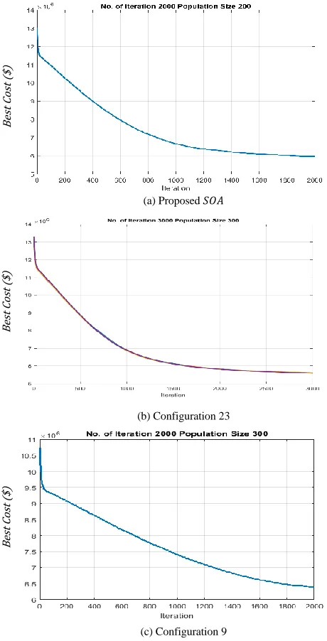
Also, the results obtained from the proposed SOA algorithm, and the GA solver associated with 𝑃𝑆, 𝑃𝑀, and 𝑃𝐿 case studies are depicted in Figure 6-Figure 8.
Best
Co
st
(
$)
(a) Proposed 𝑆𝑂𝐴
B
es
t
C
os
t
($
)
(b) Configuration 22
B
est
C
os
t (
$)
(c) Configuration 15
Figure 6 Results obtained from (a) the proposed SOA methodology, (b) the GA optimiser (𝑆22) and (c) the GA optimiser (𝑆15) for 𝑃𝑆
Best
Co
st
(
$)
(a) Proposed 𝑆𝑂𝐴
B
est
C
os
t (
$)
(b) Configuration 21
B
est
C
os
t (
$)
(c) Configuration 1
Best
Co
st
(
$)
(a) Proposed 𝑆𝑂𝐴
B
est
C
os
t (
$)
(b) Configuration 23
B
est
C
os
t (
$)
(c) Configuration 9
Figure 8 Total cost achieved from implementing (a) the proposed SOA, (b) the GA optimiser (𝑆23) and (c) the GA optimiser (𝑆9) for 𝑃𝐿
Table 18-Table 20 present the optimum quantities associated with each product family to be manufactured for consumers over the given planning horizon.
The Optimum Solution for Small-scale problem
𝑷𝟏 𝑷𝟐 𝑷𝟑 𝑷𝟒 𝑷𝟓
T1 11 1 54 4 1
T2 10 11 1 5 80
Total 21 12 55 9 81
The Optimum Solution for Medium-scale problem
𝑷𝟏 𝑷𝟐 𝑷𝟑 𝑷𝟒 𝑷𝟓 𝑷𝟔
T1 136 314 362 220 450 276
T2 391 396 292 575 403 197
T3 369 658 557 574 464 349
T4 499 656 831 433 404 509
T5 577 622 727 681 1013 1086
Total 1972 2646 2769 2483 2734 2417
The Optimum Solution for large-scale problem
𝑷𝟏 𝑷𝟐 𝑷𝟑 𝑷𝟒 𝑷𝟓 𝑷𝟔 𝑷𝟕 𝑷𝟖 𝑷𝟗 𝑷𝟏𝟎
T1 802 706 543 477 471 488 1026 768 670 590
T2 579 480 740 915 561 771 994 820 775 822
T3 710 811 917 608 877 703 952 791 946 1077
T4 1354 1128 630 1161 1058 1222 1090 1099 1427 1187
T5 1507 1771 1624 1429 1524 1229 1145 1537 1254 1554
T6 1685 1935 1762 1952 2055 1802 1848 1903 1397 1698
T7 1997 2192 2097 2037 2118 2435 1883 1918 2276 2854
T8 1904 2411 2159 2765 2271 2542 2309 2604 2437 1998
Total 10252 10371 10455 10606 10575 9608 9815 10685 10187 9990
8. Conclusion and outlook to future
In this paper, an advanced decision-making system for a class of CSN problems was proposed. A novel SOA algorithm incorporating GA as its optimisation module was designed for MPMPCSN problem. The robustness and effectiveness of the proposed methodology was verified through performing twenty-seven computational trials on three practical test problems at different granularity levels (small-scale, medium-scale, large-scale). In addition, a tuning mechanism was recommended to improve the quality of the obtained solutions that was affected by controllable parameters of the optimisation module. To this end, two statistical techniques known as ANOVA and Taguchi methods were utilised. The optimum levels associated to the controllable parameters of GA were determined as following: for 𝑷𝑺, level
1(Roulette Wheel selection), level 1 (90% crossover), level 1 (10% mutation), level 2 (120 chromosomes) and level 1 (200 iterations), respectively; for 𝑷𝑴level 2 (Tournament selection), level 2 (85%
crossover), level 1 (10% mutation), level 1 (200 chromosomes) and level 1 (500 iterations), respectively; For 𝑷𝑳 level 2
(Tournament selection), level 1 (90% crossover), level 1 (10% mutation), level 3 (300 chromosomes) and level 1 (3500 iterations), respectively. The proposed SOA was resulted in 5%, 4% and 2% improvement in total cost of CSN associated to 𝑃𝑆, 𝑃𝑀and 𝑃𝐿problems respectively, in contrast to only using GA
solver. Also, it was observed that the computational cost and time were reduced significantly.
Conflict of Interest
The authors declare no conflict of interest.
Acknowledgment
The authors are grateful to the Australian Mathematical Society (Aust MS) for providing the Lift-up fellowship which financially supported this work.
References
[1] Z. Hajiabolhasani, R. Marian, and J. Boland, "Consumer Supply Network Planning: Literature Review And Analysis," Journal of Multidisciplinary Engineering Science Studies, vol. 3, no. 3, pp. 1519-1538, 2017. [2] Z. H. Abolhasani, R. Marian, and J. Boland, "Simulation-Optimisation of
Multi-Product, Multi- Period Consumer Supply Network using Genetic Algorithms," in Intelligent Systems Conference (INTELLISYS), London,UK, 2017, pp. 34-44: IEEE, 2017.
[3] X.-S. Yang, S. Koziel, and L. Leifsson, "Computational Optimization, Modelling and Simulation: Past, Present and Future," in ICCS 2014. 14th International Conference on Computational Science, 2014, vol. 29, pp. 754–758: Procedia Computer Science.
[4] T. Hennies, T. Reggelin, J. Tolujew, and P.-A. Piccut, "Mesoscopic supply chain simulation," Journal of Computational Science, vol. 5, no. 3, pp. 463-470, 2014.
[6] N. Mustafee, K. Katsaliaki, and S. J. E. Taylor, "A review of literature in distributed supply chain simulation," presented at the Simulation Conference (WSC), 2014 Winter, 7-10 Dec. 2014, 2014.
[7] T. M. Pinho, J. P. Coelho, A. P. Moreira, and J. Boaventura-Cunha, "Modelling a biomass supply chain through discrete-event simulation∗∗This work was supported by the FCT - Fundação para a Ciência e Tecnologia through the PhD Studentship SFRH/BD/98032/2013, program POPH - Programa Operacional Potencial Humano and FSE - Fundo Social Europeu," IFAC-PapersOnLine, vol. 49, no. 2, pp. 84-89, 2016/01/01/ 2016.
[8] F. Campuzano and J. Mula, Supply chain simulation (A system dynamics approach for improving performance). Springer, 2011.
[9] G. Dellino, J. P. C. Kleijnen, and C. Meloni, "Robust optimization in simulation: Taguchi and Response Surface Methodology," Int. J. Production Economics, vol. 125, pp. 52-59, 2010.
[10] A. Huerta-Barrientos, M. Elizondo-Cortés, and I. F. d. l. Mota, "Analysis of scientific collaboration patterns in the co-authorship network of Simulation–Optimization of supply chains," Simulation Modelling Practice and Theory, vol. 46, pp. 135-148, 2014.
[11] X. Wan, J. F. Pekny, and G. V. Reklaitis, "Simulation-based optimization with surrogate models—Application to supply chain management," Computers and Chemical Engineering, vol. 29, pp. 1317–1328, 2005. [12] J. Y. Jung, G. Blaua, J. F. Pekny, G. V. Reklaitis, and D. Eversdykb, "A
simulation based optimization approach to supply chain management under demand uncertainty," Computers and Chemical Engineering, vol. 28, pp. 2087–2106, 2004.
[13] M. C. Fu, "Optimization via simulation: A review," Annals of Operations Research vol. 53, pp. 199-247, 1994.
[14] J.-H. Kang and Y.-D. Kim, "Inventory control in a two-level supply chain with risk pooling effect," International Journal of Production Economics, vol. 135, no. 1, pp. 116-124, 2012.
[15] S. M. Mousavi, A. Bahreininejad, S. N. Musa, and F. Yusof, "A modified particle swarm optimization for solving the integrated location and inventory control problems in a two-echelon supply chain network," Intell Manuf, 2014.
[16] F. T. S. Chan and A. Prakash, "Inventory management in a lateral collaborative manufacturing supply chain: a simulation study," International Journal of Production Research, vol. 50, no. 16, p. 15, 15 August 2012 2012.
[17] O. Labarthe, B. Espinasse, A. Ferrarini, and B. Montreuil, "Toward a methodological framework for agent-based modeling and simulation of supply chains in a mass customization context," Simulation Modelling Practice and Theory, vol. 15, no. 2, pp. 113-136, 2007.
[18] F. Longo and G. Mirabelli, "An advanced supply chain management tool based on modeling and simulation," Computers & Industrial Engineering, vol. 54, no. 3, pp. 570-588, 2008.
[19] A. Alrabghi and A. Tiwari, "State of the art in simulation-based optimisation for maintenance systems," Computers & Industrial Engineering, vol. 82, pp. 167-182, 4// 2015.
[20] P. Ghamisi and J. A. Benediktsson, "Feature selection based on hybridization of genetic algorithm and particle swarm optimization," IEEE Geoscience and Remote Sensing Letters, vol. 12, no. 2, pp. 309-313, 2015. [21] A. E. Eiben, R. Hinterding, and Z. Michalewicz, "Parameter control in evolutionary algorithms," IEEE TRANSACTIONS ON EVOLUTIONARY COMPUTATION, vol. 3, no. 2, pp. 124-141, 1999. [22] J. Sadeghi, S. M. Mousavi, S. T. A. Niaki, and S. Sadeghi, "Optimizing a
multi-vendor multi-retailer vendor managed inventory problem: Two tuned meta-heuristic algorithms," Knowledge-Based Systems, vol. 50, pp. 159-170, 2013.
[23] H. Ding, L. Benyoucef, and X. Xie, "Stochastic multi-objective production-distribution network design using simulation-based optimization," International Journal of Production Research, vol. 47, no. 2, pp. 479-505, 2009.
[24] A. D. Yimer and K. Demirli, "A genetic approach to two-phase optimization of dynamic supply chain scheduling," Computers & Industrial Engineering, vol. 58, no. 3, pp. 411-422, 4// 2010.
[25] A. Nikolopoulou and M. G. Ierapetritou, "Hybrid simulation based optimization approach for supply chain management," Computers & Chemical Engineering, vol. 47, pp. 183-193, 12/20/ 2012.
[26] M. Seifbarghy, M. M. Kalani, and M. Hemmati, "A discrete particle swarm optimization algorithm with local search for a production-based two-echelon single-vendor multiple-buyer supply chain," Journal of Industrial Engineering International, journal article vol. 12, no. 1, pp. 29-43, 2016. [27] E. M. Frazzon, A. Albrecht, M. Pires, E. Israel, M. Kück, and M. Freitag,
"Hybrid approach for the integrated scheduling of production and transport
processes along supply chains," International Journal of Production Research, vol. 56, 2018.
[28] J. Huang and J. Song, "Optimal inventory control with sequential online auction in agriculture supply chain: an agentbased simulation optimisation approach," International Journal of Production Research, vol. 56, no. 6. [29] S. K. Shukla, M. K. Tiwari, H.-D. Wan, and R. Shankar, "Optimization of
the supply chain network: Simulation, Taguchi, and psychoclonal algorithm embedded approach," Computers & Industrial Engineering, vol. 58, no. 1, pp. 29-39, 2// 2010.
[30] B. Unhelkar, Practical object oriented design. Thomson Social Science Press, 2005.
[31] J. Arthur F. Veinott, "Lectures in Supply-Chain Optimization," S. U. Department of Management Science and Engineering, Ed., ed. Stanford, California, 2005.
[32] B. Fahimnia, L. Luong, and R. Marian, "Genetic algorithm optimisation of an integrated aggregate production–distribution plan in supply chainsn," International Journal of Production Research, vol. 50, no. 1, pp. 81-96. [33] D. E. Goldberg, Genetic Algorithms in Search, Optimization, and Machine
Learning. MA: Addison-Wesley, 1989.
[34] N. M. Razali and J. Geraghty, "Genetic Algorithm Performance with Different Selection Strategies in Solving TSP," presented at the Proceedings of the World Congress on Engineering 2011 Vol II, London, U.K., 2011.
[35] B. Fahimnia, "An Integrated Methodology for the Optimisation of Aggregate Production-Distribution Plan in Supply Chains," Doctor of Philosophy, Mechanical and Manufacturing Engineering, University of South Australia, 2010.
[36] R. Marian, L. Luong, and K. Abhary, "Assembly sequence planning and optimisation using genetic algorithms: part I. Automatic generation of feasible assembly sequences," Applied Soft Computing vol. 2, no. 3, pp. 223-253.
[37] J.-F. Cordeau, M. Gendreau, A. Hertz, G. Laporte, and J.-S. Sormany, "New heuristics for the vehicle routing problem," in Logistic Systems: Desing and Optimization, A. Langevin and D. Riopel, Eds. United States of America: Springer, 2005, pp. 279-298.
[38] R. M. MARIAN, "Optimisation of assembly sequences using genetic algorithms," DOCTOR OF PHILOSOPHY, School of Advanced Manufacturing and Mechanical Engineering, UNIVERSITY OF SOUTH AUSTRALIA, 2003.
[39] F. T. Chan, S. Chung, and S. Wadhwa, "A hybrid genetic algorithm for production and distribution," Omega, vol. 33, no. 4, pp. 345-355, 2005. [40] Z. H. Abolhasani, R. M. Marian, and L. Luong, "Optimization of
Multi-Commodities Consumer Supply Chain- Part 1- Modelling," Journal of Computer Science, vol. 9, no. 12, p. 16, 2013.
[41] H. Xing, X. Liu, X. Jin, L. Bai, and Y. Ji, "A multi-granularity evolution based Quantum Genetic Algorithm for QoS multicast routing problem in WDM networks," Computer Communications, vol. 32, pp. 386-393, 2009. [42] C. A. C. Coello, G. B. Lamont, and D. A. V. Veldhuizen, D. E. Goldberg and J. R. Koza, Eds. Evolutionary algorithms for solving multi-objective problems, 2nd ed. (Genetic and Evolutionary Computation). New York: Springer, 2007.
[43] Jeong Hee Hong, K.-M. Seo, and T. G. Kim, "Simulation-based optimization for design parameter exploration in hybrid system: a defense system example," Simulation: Transactions of the Society for Modeling and Simulation International, vol. 89, no. 3, pp. 362-380, 2013.