Applying evolutionary optimization on the airfoil design

51 *

Corresponding author.

Email address: [email protected]

Applying evolutionary optimization on the airfoil design

Abolfazl Khalkhalia,*and Hamed Safikhanib

a_{School of Automotive Engineering, Iran University of Science and Technology, Tehran, Iran.} b_{Department of Mechanical Engineering, Amirkabir University of Technology, Tehran, Iran.}

Article info:

Received: 12/07/2012 Accepted: 15/07/2012 Online: 11/09/2012

Keywords:

Multi-objective Optimization, GMDH,

Genetic Algorithm, 4-Digit NACA Airfoils, NUMECA

Abstract

In this paper, lift and drag coefficients were numerically investigated using NUMECA software in a set of 4-digit NACA airfoils. Two metamodels based on the evolved group method of data handling (GMDH) type neural networks were then obtained for modeling both lift coefficient (CL) and drag coefficient

(CD) with respect to the geometrical design parameters. After using such

obtained polynomial neural networks, modified non-dominated sorting genetic algorithm (NSGAII) was used for Pareto based optimization of 4-digit NACA airfoils considering two conflicting objectives such as (CL) and (CD). Further

evaluations of the design points in the obtained Pareto fronts using the NUMECA software showed the effectiveness of such an approach. Moreover, it was shown that some interesting and important relationships as the useful optimal design principles involved in the performance of the airfoils can be discovered by the Pareto-based multi-objective optimization of the obtained polynomial meta-models. Such important optimal principles would not have been obtained without using the approach presented in this paper.

Nomenclature

CD Drag Coefficient

CL Lift Coefficient

CP Pressure Coefficient

AoA Airfoil Angle of Attack

Re Reynolds Number.

X* Vector of Optimal Design Variables

F(x) Vector of Objective Function

pF* Pareto Front

P* Pareto Set

MO Multi-Objective

GMDH Group Method of Data Handling

SVD Singular Value Decomposition

NSGA Non-dominate Sorting Genetic Algorithm

GA Genetic Algorithm

1. Introduction

52

Razaghi et al. [2] investigated a multi-objective optimization process to NACA 0015 airfoil with a synthetic jet and at a constant angle of attack and tried to maximize CL and minimize

CD; they finally presented 5 sets of optimum

design variables, from among which the designer can select one. Both of the above mentioned studies were performed at a constant angle of attack; but, angle of attack was one of the design variables in the present study.

Optimization of airfoils is indeed a multi-objective optimization problem rather than a single-objective optimization problem that has been considered so far in the literature. Both CL

and the CD in airfoils are important objective

functions to be optimized simultaneously in such a real world complex multi-objective optimization problem. These objective functions are either obtained from experiments or computed using very timely and high-cost computer fluid dynamic (CFD) approaches, which cannot be used in an iterative optimization task unless a simple but effective meta-model is constructed over the response surface according to the numerical or experimental data. Therefore, modeling and optimization of the parameters were investigated in the present study using GMDH-type neural networks and multi-objective genetic algorithms in order to maximize the lift and minimize the drag coefficients.

System identification and modeling of complex processes using input-output data have always attracted many research efforts. In fact, system identification techniques are applied in many fields in order to model and predict the behaviors of unknown and/or very complex systems based on given input-output data [3]. Thus, soft-computing methods [4], which are concerned with computation in an imprecise environment, have gained significant attention. The main components of soft computing, namely, fuzzy logic, neural network and evolutionary algorithms have shown great ability in solving complex non-linear system identification and control problems. Many efforts have been made to use evolutionary methods as effective tools for system identification [5].

Among these methodologies, Group Method of Data Handling (GMDH) algorithm is a self-organizing approach by which gradually complicated models are generated based on the evaluation of their performances on a set of multi-input-single-output data pairs (X_i,y_i)

(i=1, 2, …, M). The GMDH was first developed by Ivakhnenko [6] as a multivariate analysis method for modeling and identification of complex systems, which can be used to model complex systems without having specific knowledge of the systems. The main idea of GMDH is to build an analytical function in a feed forward network based on a quadratic node transfer function [7], the coefficients of which are obtained using regression technique. In recent years, however, the use of such self-organizing networks has led to successful application of the GMDH-type algorithm in a broad range of areas in engineering, science and economics [6].

53 In this paper, CL and CD in a set of 4-digit

NACA airfoils were numerically investigated using CFD techniques. The validations of results were achieved by comparing the results obtained in this research versus the experimental data of Abbott and Vondoenhoff [12]. Next, genetically optimized GMDH type neural networks were used to obtain polynomial models for the effects of geometrical parameters of the airfoils and the angle of attack on both CL and CD. Such an approach of

meta-modeling of those numerical results allowed for iterative optimization techniques to design the airfoils optimally and affordably in computational terms. The obtained simple polynomial models were then used in a Pareto based multi-objective optimization approach to find the best possible combinations of CL and

CD, known as the Pareto front.

2. Numerical Simulation of Airfoils

2.1. Numerical Scheme

The governing equations of incompressible flow are as follows:

• Continuity equation:

0 i i V x ∂ =

∂ (1)

• Reynolds averaged momentum equation:

2

1

i i

i j

i j j j

DV p V

u u

Dt ρ x ν x x x

∂

∂ ∂

= − + −

∂ ∂ ∂ ∂ (2)

• Standard k–ε _{model used for turbulence} modeling: k C x V u u k C x k C x Dt D x V u u x k k C x Dt Dk j i j i j k j j i j i i k j 2 2 1 2 2 ] ) [( ] ) [( ε ε ε ν ε ε ν ε ε

ε _∂∂ −

− ∂ ∂ + ∂ ∂ = ∂ ∂ − ∂ ∂ + ∂ ∂ = (3)

The simulations were performed using NUMECA software. First, one airfoil was modeled in Auto blade 3.6 and then the Design 2D environment of NUMECA could automatically generate the database with different design variables. For For CFD grid generation, the Auto Grid environment of Numeca was coupled with the Auto Blade

environment. A structured C-type grid system was used for the calculation of the flow field around the airfoils. The computational domain is shown in Fig. 1.

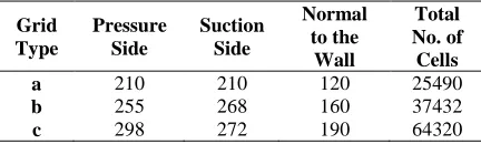
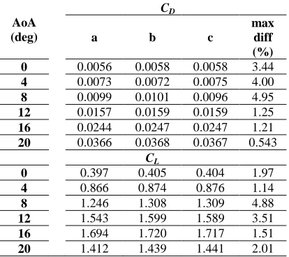
To test grid independency, three grid types (named a, b and c) with increasing grid density were studied and their details are listed in Table 1. The computational results of 3 grid types for different angles of attack are compared in Table 2. As can be seen, the maximum difference between the results was less than 5%; so the grid type (a) was used for all computations in the present study. On the outer boundary, the uniform flow boundary conditions were imposed on the upstream boundary and the right (outflow) boundary condition was set to a zero velocity gradient condition [2]. A no-slip wall boundary condition was taken on the airfoil surface. The simulations were performed under Reynolds number2×106.

Table 1. Details of 3 grid types used in grid

independency test around NACA 4412.

Grid Type Pressure Side Suction Side Normal to the Wall Total No. of Cells

a 210 210 120 25490

b 255 268 160 37432

c 298 272 190 64320

2.2. Definition of the Design Variables

The design variables in the present study were the maximum camber height as percentage of chord length (x1), the maximum camber

location as percentage of chord length (x2) and

the angle of attack (x3). The design variables

54

2.3. Validation of the CFD Results

The number of 324 various CFD runs were performed due to those different design geometrics. The samples of numerical results using CFD are shown in Table 4. To attain confidence about the simulation, it is necessary to compare the CFD results with the experimental data.

Table 2. Comparison of CL and CD for 3 grid types around NACA 4412.

AoA (deg)

CD

a b c

max diff (%)

0 0.0056 0.0058 0.0058 3.44

4 0.0073 0.0072 0.0075 4.00

8 0.0099 0.0101 0.0096 4.95

12 0.0157 0.0159 0.0159 1.25

16 0.0244 0.0247 0.0247 1.21

20 0.0366 0.0368 0.0367 0.543

CL

0 0.397 0.405 0.404 1.97

4 0.866 0.874 0.876 1.14

8 1.246 1.308 1.309 4.88

12 1.543 1.599 1.589 3.51

16 1.694 1.720 1.717 1.51

20 1.412 1.439 1.441 2.01

Table 3. Design variables and their range of

variations.

Design Variable From To

Maximum camber height as

percentage of chord length (x1 ) 1 9

Maximum camber location as percentage of chord length (x2 )

1 8

Angle of attack (x3) 0o 20o

Figure 3 shows the computed lift coefficient versus angle of attack compared with the experimental data. As can be observed in this figure, the computed result was reasonably close to the graph which was experimentally obtained. The stall angle was overestimated by 2 % and the maximum CL by 3 % because, in

general, there exists a difficulty for numerical approaches to match the lift coefficient for angles of attack above the separation angle [13]. The comparison between numerical and experimental pressure coefficient (CP) is shown

in Fig. 4. It is obvious that numerical

simulations can properly adapt with the pattern of experimental CP curve.

Fig. 1. Schematic representation of computational

grid.

Fig. 2. Definition of design variables.

Table 4. Samples of numerical results using CFD.

Num

Input Data Output Data

x1 x2 x3(deg) CL CD

1 6 2 0 0.687 0.0061

2 9 2 0 1.024 0.0066

3 3 4 4 0.874 0.0072

4 7 3 4 1.321 0.0069

5 5 1 8 1.395 0.0094

6 5 6 8 1.491 0.0115

7 1 3 12 1.541 0.0141

8 5 8 12 1.539 0.0212

9 9 2 16 1.341 0.0278

10 5 6 16 1.661 0.0271

…

323 9 8 20 1.451 0.0567

324 4 8 20 1.495 0.0461

The results obtained in such CFD analysis can now be used to build the response surface of both CD and CL for those different 324

55 neural networks. Such meta-models will, in

turn, be used for the Pareto-based multi-objective optimization of the 4-digit NACA airfoils. A post analysis using the CFD was also performed to verify optimum results using the meta-modeling approach. Finally, the solutions obtained by the approach of this paper exhibited some important trade-offs among those objective functions which can be simply used by a designer to optimally compromise among the obtained solutions.

Fig. 3. Comparison of numerical and experimental

[12] results for CD versus angle of attack around NACA 4412.

Fig. 4. Comparison of numerical and experimental

[12] results for CL around NACA 4412 at angle of attack 8o.

3. Modeling of CL and CD using GMDH-type

neural network

By means of GMDH algorithm, a model could be represented as a set of neurons in which different pairs of each layer were connected through a quadratic polynomial and thus new neurons were produced in the next layer. Such representation can be used in modeling in order to map inputs to outputs. The formal definition of the identification problem was to find a function fˆ_{which can be approximately used} instead of actual one,f _{in order to predict} output yˆ for a given input vector

( , , , ..., )

1 2 3

X x x x x

n =

as close as possible to its actual output y. Therefore, given M observation of multi-input-single-output data pairs so that:

( , , , ..., )

1 2 3

y f x x x x

i = i i i in (i=1, 2… M), (4) It is now possible to train a GMDH-type neural network to predict the output values

i

yˆ for any

given input vector as:

1 2 3

( , , , ..., )

i i i in

X = x x x x , that is:

ˆ

ˆ ( , , , ..., )

1 2 3

y f x x x x

i = i i i in (i=1, 2… M), (5)

The problem is now to determine a GMDH-type neural network so that the square of difference between the actual output and the predicted one is minimized, that is:

2 ˆ

[ ( , , , ..., ) ] min

1 2 3

1

M

f x x x x y

i i i in i

i

∑ _{− →}

= (6)

General connection between inputs and output variables can be expressed by a complicated discrete form of the Volterra functional series in the form of:

0

1 1 1

n n n

y a a x_{i i} a_ijx x_{i j}

i i j

∑ ∑ ∑

= + +

= = =

...

1 1 1

n n n

a_ijk x x_{i j}x_k i j k

∑ ∑ ∑ ₊

= = =

56

where … is known as the Kolmogorov-Gabor polynomial [7]. This full form of mathematical description can be represented by a system of partial quadratic polynomials consisting of only two variables (neurons) in the form of:

ˆ ( , ) _{0 1 2}

y =G x_i x _j =a +a x_i +a x _j

2 2

5

3 4

a x x_{i j} a x_i a x_j

+ + + (8) There are two main concepts involved in the design of GMDH-type neural networks, namely, the parametric and the structural identification problems. In this way, some authors have presented a hybrid GA and singular value decomposition (SVD) method to optimally design such polynomial neural networks [8]. The methodology in these references was successfully used in this paper to obtain the polynomial models of CL and CD.

The obtained GMDH-type polynomial models showed very good prediction ability of unforeseen data pairs during the training process, which will be presented in the following sections.

Fig. 5. CFD versus Network for drag coefficient.

The input–output data pairs used in such modeling involved two different data tables obtained from CFD simulation discussed in Section 2. Both of the tables consisted of three variables as inputs, namely, the geometrical parameters of the airfoils, maximum camber

(x1), location of maximum camber (x2) and

angle of attack (x3), and outputs, which were CL

and CD. The tables consisted of the total of 324

patterns, which were obtained from the numerical solutions to train and test such GMDH type neural networks.

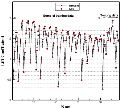
Fig. 6. CFD versus Network for lift coefficient.

However, in order to demonstrate the prediction ability of the evolved GMDH type neural networks, the data in both input–output data tables were divided into two different sets, namely, training and testing sets. The training set, which consisted of 304 out of the 324 input–output data pairs for CD and CL, was used

for training the neural network models. The testing set, which consisted of 20 unforeseen input–output data samples for CD and CL during

the training process, was merely used for testing in order to show the prediction ability of such evolved GMDH type neural network models.

The GMDH type neural networks were then used for such input–output data to find the polynomial models of CD and CL with respect to

their effective input parameters. In order to genetically design such GMDH type neural networks described in the previous section, the population of 10 individuals with crossover probability (Pc) of 0.7 and mutation probability (Pm) of 0.07 wasn used in 500 generations for CD and CL. The corresponding polynomial

57

2

1 0.018 0.0001 1 -0.0017 2-4.7e-6 1

Y = + x x x

2

2 1 2

+0.0002x +0.0001x x (9a)

2

1 3 1

0.013-0.95 -0.001 30.45

D

C = Y x + Y

2

3 1 3

+9.81e-005x + 0.072Y x (9b) Similarly, the corresponding polynomial representation of the model for CL is in the form

of:

2

1 0.715 0.0819 1 0.167 2-0.0054 1

Y ′= + x + x x

2

2 1 2

-0.0178x + 0.0034 x x (10a)

2

2 0.178 0.212 2 0.1454 3-0.0173 2

Y ′ = + x + x x

2

3 2 3

-0.00441x -0.0021x x (10b)

2

3 0.006 0.169 1 0.163 3-0.0066 1

Y ′ = + x + x x

2

3 1 3

-0.0043x -0.0062 x x (10c)

2

4 -5.770 12.50 1-0.572` 1-5.6882 1

Y ′= + Y′ x Y ′

2

1 1

-0.0165 x +0.5824 x Y ′ (10d)

2

2

5 0.1930 -0.5041Y2 1.232Y -0.3342Y 3

Y ′= ′+ ′ ′

2

3 3 2

-1.0680Y′ +1.507Y Y′ ′ (10e)

2

4 5 4

-1.661 2.015Y 0.973Y -0.424Y

L

C = + ′+ ′ ′

2

5 4 5

0.1647Y -0.2950 Y Y′ ′ ′

+ (10f) The very good behavior of such a GMDH type neural network model for CD is also depicted in

Fig. 5, for both the training and testing data. Such a behavior is also shown for the training and testing data of CL in Fig. 6. It is evident that

the evolved GMDH type neural network in terms of simple polynomial equations successfully model and predict the outputs of the testing data that have not been used during the training process. The models obtained in this section can be utilized in a Pareto multi-objective optimization of the airfoil considering both CD and CL as conflicting objectives. Such a

study may unveil some interesting and important optimal design principles that would not have been obtained without using a multi-objective optimization approach.

4. Multi-Objective Optimization

Multi-objective optimization, which is also called multi criteria optimization or vector optimization, has been defined as finding a

vector of decision variables satisfying constraints to give acceptable values to all objective functions [14]. In these problems, there are several objective or cost functions (a vector of objectives) to be optimized (minimized or maximized) simultaneously. These objectives often conflict with each other so that improving one of them will deteriorate another. Therefore, there is no single optimal solution as the best with respect to all the objective functions. Instead, there is a set of optimal solutions, known as Pareto optimal solutions or Pareto front [15], for multi-objective optimization problems.

The concept of Pareto front or set of optimal solutions in the space of objective functions in multi-objective optimization problems (MOPs) stands for a set of solutions that are non-dominated to each other but are superior to the rest of the solutions in the search space. This means that it is not possible to find a single solution to be superior to all other solutions with respect to all objectives so that changing the vector of design variables in such a Pareto front consisting of these non-dominated solutions could not lead to the improvement of all objectives simultaneously.

Consequently, such a change will lead to deterioration of at least one objective. Thus, each solution of the Pareto set includes at least one objective inferior to that of another solution in that Pareto set although both are superior to others in the rest of search space. Such problems can be mathematically defined as:

Find the vector * * * *

1, 2, ...,

T n

X =_x x x _ to optimize:

[

1 2

]

( ) ( ), ( ), ..., _k( ) T

F X = f X f X f X , (11) Subject to m inequality constraints:

( ) 0 , i 1 to m i

g X ≤ = , (12) And p equality constraints:

( ) 0 , j 1 to p

j

h X = = , (13) where X *∈ ℜn _{is the vector of decision or}

58

multi-objective minimization based on Pareto approach can be conducted using some definitions.

4.1. Definition of Pareto Dominance

A vector U =

[

u u₁, ₂, ...,u_k

]

∈ ℜk is dominant to vector V =

[

v v₁, ₂, ...,v_k

]

∈ ℜk (denoted by

U _pV ) if and only if ∀ ∈i

{

1, 2, ...,k

}

, u_i ≤v_i

∧ ∃ ∈j

_{

1, 2, ...,k

_}

: uj<vj. In other words, there is at least one u_j which is smaller than

j

v while the remaining

u

s are either smaller or equal to the corresponding

v

s .

4.2. Definition of Pareto Optimality

A point *

X ∈ Ω ( Ω is a feasible region in n

ℜ

satisfying Eq. (12 and 13) is said to be Pareto optimal (minimal) with respect to all X ∈ Ω if and only if *

( ) ( )

F X pF X . Alternatively, it can be readily restated as:

}

{

1, 2, ...,

i k

∀ ∈ , *

{ }

X X

∀ ∈ Ω − *

( ) ( )

i i

f X ≤f X ∧ ∃ ∈j

{

1, 2, ...,k

}

:

*

( ) ( )

j j

f X <f X .

In other words, the solution *

X is said to be Pareto optimal (minimal) if no other solution can be found to dominate *

X using the definition of Pareto dominance.

4.3. Definition of a Pareto Set

For a given MOP, a Pareto set Ƥ٭_{is a set in the} decision variable space consisting of all the Pareto optimal vectors as:

Ƥ٭={X ∈ Ω|∄X′∈ Ω: (F X′)_pF X( )}

In other words, there is no other X ′ as a vector of decision variables in Ωthat dominates any X ∈Ƥ٭_.

4.4. Definition of a Pareto Front

For a given MOP, the Pareto front ƤŦ٭ _{is a set} of vector of objective functions which are obtained using the vectors of decision variables in the Pareto set Ƥ٭_{; i.e.:}

ƤŦ٭

1 2

{ (F X ) ( (f X ),f (X ),....,f_k(X)):X

= = ∈Ƥ٭_}

In other words, the Pareto front ƤŦ٭ _{is a set of} the vectors of objective functions mapped from Ƥ٭_.

Evolutionary algorithms have been widely used for multi-objective optimization because of their natural properties suited for these types of problems. This is mostly because of their parallel or population-based search approach. Therefore, most of the difficulties and deficiencies within the classical methods in solving multi-objective optimization problems are eliminated. For example, there is no need for either several runs to find the Pareto front or quantification of the importance of each objective using numerical weights.

In this way, the original non-dominated sorting procedure given by Goldberg [16] is the catalyst for several different versions of multi-objective optimization algorithms [17]. However, it is very important that the genetic diversity within the population be preserved sufficiently. This main issue in MOPs has been addressed by many related studies [18]. In this paper, the premature convergence of MOEAs was prevented and the solutions were directed and distributed along the true Pareto front using a recently developed algorithm, namely, the є -elimination diversity algorithm by some of the authors [9‒_11].

5. Multi-Objective optimization of 4-Digit NACA airfoils using polynomial neural network models

59 simultaneously optimized with respect to the

design variables, x1, x2 and x3 (Fig. 2). The

multi-objective optimization problem can be formulated in the following form:

Maximize CL= f1 (x1, x2, x3)

Minimize CD= f 2(x1, x2, x3) (14)

1<x1<9 (14)

Subject to: 1<x2<8

0o<x3<20 o

The evolutionary process of Pareto multi-objective optimization was accomplished using the recently developed NSGA II algorithm, namely the є_{-elimination diversity algorithm [8} and 10], in which the population size of 60 was chosen in all runs with crossover probability of Pc and mutation probability of Pm as 0.7 and

0.07, respectively.

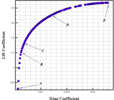
Figure 7 depicts the obtained non-dominated optimum design points as a Pareto front of those two objective functions. There were five optimum design points, namely, A, B, C, D and E, the corresponding design variables and objective functions of which are shown in Table 5. Moreover, for more clarity, the pressure contours of optimum design points (airfoil number plus angle of attack) are shown in Fig. 8. These points clearly demonstrate the tradeoffs in objective functions CD and CL from

which an appropriate design can be compromisingly chosen.

It is clear from Fig. 7 that all the optimum design points in the Pareto front are non-dominated and could be chosen by a designer as the optimum airfoil. Evidently, choosing a better value for any objective function in the Pareto front would cause a worse value for another objective. The corresponding decision variables of the Pareto front shown in Fig. 7 were the best possible design points so that, if any other set of decision variables is chosen, the corresponding values of the pair of objectives will locate a point inferior to this Pareto front. Such an inferior area in the space of the two objectives is in fact bottom/right side of Fig. 7.

In Fig. 7, the design points A and E stand for the best CD and CL , respectively. Moreover, the

other optimum design points B and D can be simply recognized from Fig. 7.

The design point B exhibits important optimal design concepts. In fact, optimum design point B obtained in this paper exhibits an increase in CD (about 3.46%) in comparison with that of

point A while its CL improves by about 42.4%.

Similarly, optimum design point D exhibits a decrease in CL (about 14.25%) in comparison

with that of point E while its CD improves by

about 62.6% in comparison with that of point E. It is now desired to find trade-off optimum design points which compromise both objective functions. This can be achieved by the method employed in this paper, namely, the mapping method. In this method, the values of objective functions of all non-dominated points were mapped into intervals 0 and 1.

Fig. 7. Pareto front of lift and drag coefficients for

4-digit NACA airfoils.

Table 5. Design variables and objective functions

values of Pareto points.

Design

Points x1 x2 x3

(deg) CD CL

A 2 3 2.75 0.0056 0.7188

B 6 3 3.51 0.0062 1.2066

C 7 4 4.01 0.0068 1.3256

D 8 4 9.04 0.0121 1.7058

E 8 5 13.84 0.0229 1.8692

60

one with the minimum sum of those values. Consequently, the optimum design point C was the trade-off points obtained from the mapping method.

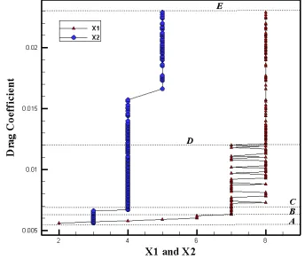
There were some interesting design facts which can be used in the design of such airfoils. It is clear from Fig. 9 that there was a quadratic relation between CD and angle of attack (x3).

Variations of x1 and x2 corresponding to the

Pareto front of CD and CL are shown in Fig.10

and 11, respectively.

As seen from these figures, from point A to B, x1 varies almost linearly whereas x2 is constant;

similarly, from point B to C, x1 and x2 are

constant. From point C to D, x1 oscillates

between values 7 and 8 whereas x2 is constant.

Finally, from point D to E, x1 is almost constant

whereas x2 has two values of 4 and 5. These

useful relationships that are indefeasible between the optimum design variables of 4-digit NACA airfoils could not be discovered without the use of multi-objective Pareto optimization process presented in this paper.

Fig. 8. Pressure contour of optimum points.

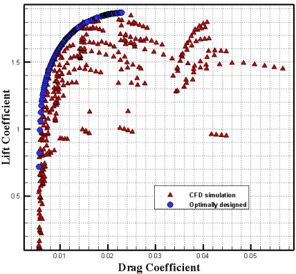
The Pareto front obtained from the GMDH-type neural network model (Fig. 7) was superimposed with the corresponding CFD

simulation results in Fig. 12. It can be clearly seen from this figure that the Pareto front obtained in this way is placed on the best possible combination of the objective values of CFD data, which demonstrates the effectiveness of this paper both in deriving the model and in obtaining the Pareto front.

In a post numerical study, the design points of the obtained Pareto front were re-evaluated by CFD. It should be noted that the optimum design points of the Pareto set were not included in the training and testing sets utilized meta-modeling using GMDH-type neural network, which made such re-evaluation sensible. The results of such CFD analysis re-evaluations were compared with those of numerical results using the GMDH model, as shown in Table 6. As can be seen, the GMDH data agreed well with the CFD results.

Fig. 9. Optimal quadratic relation of CD with respect to angle of attack (x3).

61

Table 6. Re-evaluation of the obtained optimal Pareto front using CFD.

Points CD-GMDH CD-CFD Error (%) CL-GMDH CL-CFD Error (%)

A 0.0056 0.0059 5.91 0.7188 0.7620 5.68

B 0.0062 0.0065 5.08 1.2066 1.2439 3.11

C 0.0068 0.0069 2.54 1.3256 1.3909 4.70

D 0.0121 0.0125 3.69 1.7058 1.7540 2.81

E 0.0229 0.0239 4.51 1.8692 1.9450 3.90

Fig.11. Optimal variation of CL with respect to x1 and x2.

Fig. 12. Overlay graph of the obtained optimal

Pareto front with the CFD data.

6. Conclusions

Genetic algorithms were successfully used both for optimal design of generalized GMDH type neural networks models of CL and CD in 4-digit

NACA airfoils and for multi-objective Pareto based optimization of such processes. Two different polynomial relations for CL and CD

were found by the evolved GS-GMDH type neural networks using some experimentally validated CFD simulations for input–output data of the airfoils.

The derived polynomial models was then used in an evolutionary multi-objective Pareto based optimization process so that some interesting and informative optimum design aspects were revealed for airfoils with respect to the control variables of airfoils, geometrical parameters of x1, x2 and angle of attack (x3). Consequently,

some very important trade-offs in the optimum design of airfoils were obtained and proposed based on the Pareto front of two conflicting objective functions. Such combined application of GMDH type neural network modeling of input–output data and subsequent non-dominated Pareto optimization process of the obtained models could be very promising in discovering useful and interesting design relationships.

References

[1] A. Oyama, T. Nonomura and K. Fujii, “Data Mining of Pareto-Optimal Transonic Airfoil Shapes Using Proper Orthogonal Decomposition”, Journal of Aircraft, Vol. 47, No. 5, pp. 1756-1762, (2010).

Multi-62

Objective Optimization of Stall Control on NACA 0015 Airfoil with a Synthetic Jet Using GMDH Type Neural Networks and Genetic Algorithms”, IJE Transactions A: Basics, Vol. 22, No.1, pp. 69‒_{88, (2009).}

[3] K. J. Astrom, and P. Eykhoff, “System identification, a survey”, Automatica, Vol. 7, pp. 123‒_{162, (1971).}

[4] E. Sanchez, T. Shibata and L. A. Zadeh, Genetic Algorithms and Fuzzy Logic Systems, Vol. 7, World Scientific, Riveredge, NJ, (1997).

[5] K. Kristinson and G. Dumont, “System identification and control using genetic algorithms”, IEEE Trans. On Sys., Man, and Cybern, Vol. 22, No. 5, pp. 1033‒_{1046, (1992).}

[6] A. G. Ivakhnenko, “Polynomial Theory of Complex Systems”, IEEE Trans. Syst. Man & Cybern, SMC-1, pp. 364‒_378, (1971).

[7] S. J. Farlow, Self-organizing Method in Modeling: GMDH type algorithm, Marcel Dekker Inc., New York, (1984). [8] N. Nariman-Zadeh, A. Darvizeh, M. E.

Felezi and H. Gharababaei, “Polynomial modelling of explosive compaction process of metallic powders using GMDH-type neural networks and singular value decomposition”, Model. Simul. Mater. Sci. Eng., Vol. 10, No.6, pp.727‒_{744, (2002).}

[9] A. Khalkhali and Hamed Safikhani, “Pareto Based Multi-Objective Optimization of Cyclone Vortex Finder using CFD, GMDH Type Neural Networks and Genetic Algorithms”, Engineering Optimization, Vol. 44, No. 1, pp. 105‒_{118, (2012).}

[10] A. Khalkhali, Mehdi Farajpoor, Hamed Safikhani, “Modeling and Multi-Objective Optimization of Forward-Curved Blades Centrifugal Fans using CFD and Neural Networks”, Transaction

of the Canadian Society for Mechanical Engineering, Vol. 35, No. 1, pp. 63-79, (2011).

[11] K. Atashkari, N. Nariman-Zadeh, M. Go¨lcu, , A. Khalkhali and A. Jamali “Modeling and multi-objective optimization of a variable valve timing spark-ignition engine using polynomial neural networks and evolutionary algorithms”, Energy Conversion and Management, Vol. 48, No. 3, pp.1029– 41, (2007).

[12] H. Abbott and A. E. Von Doenhoff, Theory of Wing Sections, Dover Publications, New York, pp. 61‒62, (1958).

[13] W. K. Anderson, J. L. Thomas and C. L. Rumsey, “Application of Thin-Layer Navier Stokes Equations near Maximum Lift”, AIAA Journal, Vol. 13, pp. 49-57, (1984).

[14] C. A. Coello and A. D. Christiansen “Multi objective optimization of trusses using genetic algorithms”, Computers & Structures, Vol. 75, pp. 647‒_{660, (2000).} [15] V. Pareto, Cours d’economic ploitique,

Lausanne, Rouge, (1896).

[16] D. E. Goldberg, Genetic Algorithms in Search, Optimization, and Machine Learning, 1st ed., Addison-Wesley, New York, (1989).

[17] C. M. Fonseca and P. J. Fleming, “Genetic algorithms for multi-objective optimization: Formulation, discussion and generalization”, Proc. of the Fifth Int. Conf. on Genetic Algorithms, Forrest S. (Ed.), San Mateo, CA, Morgan Kaufmann, pp. 416‒_{423, (1993).}