Comparative Analysis of MIT Rule and
Differential Evolution on Magnetic Levitation
System
Priyank Jain and M. J. Nigam
Indian Institute of Technology, Roorkee, India Email: {priyankjain.gsits, mkndnfec}@gmail.comAbstract—In high accuracy applications such as designing autopilot system for aircrafts, missile guiding systems and in various fields for robotics and automation, one needs to design the control system with more powerful and advanced techniques so as to maintain the satisfactory performance of the overall system. The paper presents the comparative analysis of MIT rule based control with Differential Evolution (DE) algorithm based control by implementing them on magnetic levitation system in real time. It also shows the development of adjustment mechanism with necessary mathematics using gradient algorithm based MIT rule along with the mathematical modeling of magnetic levitation system. The simulations have been performed using MATLAB, and a comparative study among two strategies has been done based on these simulations. The performance of the developed controllers has been evaluated on magnetic levitation system in real time, which suggests that DE based offline tuned PID controller performs comparatively better than MIT rule based online tuned PID controller. Results also depict that MIT rule control is very sensitive to parameter variations, whereas DE based control shows robust performance.
Index Terms—adaptive control, differential evolution, magnetic levitation, MIT rule, PID controller
I. INTRODUCTION
Inherent disturbances and inaccuracies lead to parameter variations in any physical system which may result in degradation in the performance and sometimes damage the system. In high accuracy applications such as designing autopilot systems for aircrafts, missile guiding systems and in various fields for robotics and automation, one needs to design the control system with more powerful and advanced techniques so as to maintain the satisfactory performance of the overall system. Adaptive Control is one of the widely used advanced control strategies, in which one needs to design an adjustment mechanism to alter the adjustable parameters of controller [1]. Gradient theory based MIT rule is one of them, which uses the concept of altering the adjustable parameters of conventional PID controller in the direction so that the error between plant output and reference input can be minimized [1]-[3]. This type of control is also called online tuned PID control. Online tuning results in
Manuscript received February 19, 2014; revised May 20, 2014.
non-linear behavior of the overall control system which results in good performance where nonlinearities and disturbances are inherent part of the system [4].
Another approach to automatically tune the parameters of conventional controller is Differential Evolution Soft Computing Algorithm widely known as DE algorithm [5]. This technique uses a population based search algorithm to estimate the controller parameters so as to minimize the integral square error (ISE) and this estimation is done automatically through writing a program using MATLAB [5]-[8]. DE based PID tuning comes under offline tuning methods which sets the values of PID parameters based on a performance index before the simulation starts [6].
The performance of both strategies has been evaluated on magnetic levitation system implemented in real time. Mathematical linear modeling of magnetic levitation system is shown in section II along with the schematic diagram of the system [9]. Later sections explain strategies, simulations and results with necessary mathematics and graphs.
II. MAGNETIC LEVITATION SYSTEM
Magnetic levitation systems are widely used in various fields, such as frictionless bearings, high speed maglev passenger trains, levitation of wind tunnel models, magnetic levitation anti-vibration systems, etc. Magnetic levitation is a typical nonlinear complex system in which the uncertainty of the system is mainly due to modeling error, electromagnetism interfere and other outside disturbances [9]. There is only one steady state of the magnetic levitation system, which is, when the electromagnetic force balance the gravity force of the levitating object [9].
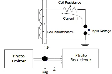
Fig. 1 shows the schematic diagram of magnetic levitation system where,
u: Input voltage
i: Current in the coil of electromagnet R: Coil’s resistance
L: Coil’s inductance
Assuming the ball is not disturbed by external forces, the dynamic equation in vertical direction can be described as,
̈ (1)
In (1), F is force due to magnetic field,
F = ⁄ (2)
then,
̈ ⁄ (3)
where,
Magnetic Field Constant k=-0.25μ0AN2Kf ‘m’ is mass of ball,
‘g’ is acceleration due to gravity, ‘i’ is the current through the coil, ‘N’ is no. of turns in the coil, ‘R’ is the resistance
‘A’ is the cross sectional area of the coil, and ‘x’ is the position of the ball levitating in the air.
In (3), let us assume the state parameters x1 and x2 as,
1=
2= ̇ Hence, the state equations will be,
̇1= 2 (4)
̇2= ⁄ (5)
To linearize (5), we will use small signal linearization around the operating point x=x0 and i=i0.
TABLE I. VARIOUS PARAMETERS OF MAGNETIC LEVITATION
SYSTEM
Parameter Value Parameter Value
Mass of the ball: m 22gms Operating Position: x0
20 mm
Radius of the ball: r 12.5mm Operating Current: i0
0.6105 A
Resistance of the coil:
R 13.8Ώ Constant: k
2.314*10-4
Nm2/ A2
According to small signal linearization,
If ̇=f(x, i) where f shows a non-linear relationship, then
̇= { │ at operating pt.} x + {
│at operating pt.} i (6)
Applying (6), we will get the following linear state equations,
̇1= 2 (7)
̇2=
( ) 1
( ) (8)
Various values used for simulations have been shown in the Table 1 give below. Here, it is noticeable that the operating point (x0, i0) of the magnetic levitation system indicates that it generates i0=0.61A of currents to levitate the ball in the air at x0=20mm [9].
Using values of various parameters shown in Table I and converting the state space equations represented by (7) and (8) into transfer function form, we will get the relationship between position and current (in terms of voltages) as shown below,
G(s)= ⁄
G(s) =
⁄ (9)
III. MITRULE
MIT rule was first developed and used in Massachusetts Institute of Technology for designing the autopilot systems for aircrafts [3]. MIT rule is based on the gradient theory which uses the alteration of controller parameters in the negative direction of gradient of a cost function [10]. This cost function is defined in terms of the error between the actual behavior and ideal behavior of the plant.
Defining the cost variable,
2
/2 (10)
In (10), e is the error between plant output and reference model output, and k is the adjustable parameter of the controller.
Applying gradient theory [11],
(11)
Using the gradient theory, we will get the following equation which depicts the relationship between the change in parameter k with error e(t) [3].
(12)
Hence the adjustment law developed by the equation given above using Laplace transform will be,
(13)
where represents the Laplace transformation and ‘s’ represents the Laplace variable.
The adjustment mechanism developed by (13) will be as shown in Fig. 2. The adjustment mechanism shown in Fig. 2 can be used anywhere in the controller to adjust the parameters [12]. Although, using this mechanism with a feedback controller may not be justified in some cases but the developed controller with it works fine and produces satisfactory results.
IV. DIFFERENTIAL EVOLUTION ALGORITHM
introduced by Storn and Price in 1996 to solve the Chebychev Polynomial fitting problem used in filter designing [13]. The decisive idea behind DE is an arrangement for producing trial parameter vectors and the selection of these vectors is based on heuristic optimization [14], [15].
Typical parameters used in DE are listed below;
D–problem dimension
N–No. of Population
CR–Crossover Probability
F–Scaling Factor
G–Number of generation/stopping condition
L, H–boundary constraints
Figure 2. Adjustment Mechanism of Model Reference Adaptive Controller using MIT rule
Storn and Price have shown some rules in selecting the control parameters in their first research paper published in 1996 [5], [8]. Theses rule are described with details in [13] and shown below with brief description;
Step 1. Initialization:
(i) Define upper and lower boundaries [L, H] and initialize all DE parameters.
(ii) Initialize parameter vectors over lower and upper limits,
i,G = [ 1,i,G , 2,i,G , ... D,i,G]; i = 1, 2, ..., N. Step 2. Mutation:
(i) For a given parameter vector i,G randomly select three vectors p,G, q,G and r,G such that the indices ‘i’, ‘p’, ‘q’ and ‘r’ are distinct.
(ii) Add the weighted difference of two of the vectors to the third,
i,G+1 = p,G + F( q,G – r,G) (14)
The mutation factor F is a constant from [0, 2] and
i,G+1 is called the donor vector.
Step 3. Recombination:
(i) Recombination incorporates successful solutions from the previous generation. The trial vector i,G+1 is developed from the elements of the target vector, i,G, and the elements of the donor vector, i,G+1.
(ii) Elements of the donor vector enter the trial vector with probability CR,
i,G+1 = {
(15) i = 1, 2, ..., N; j = 1, 2, ..., D
Step 4. Selection:
The target vector is compared with the trial vector
i,G+1 and the one with the lowest function value is
admitted to the next generation.
i,G+1 = {
(16)
V. SIMULATIONS
A. Using MIT Rule Based Controller
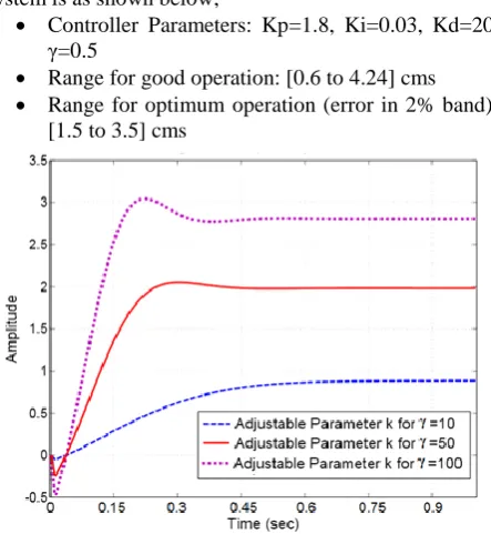
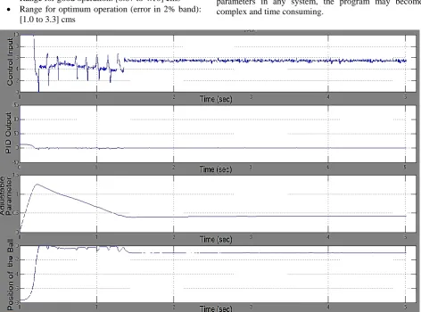
Simulations have been performed on MATLAB and are shown in this section. Fig. 3 and Fig. 4 show the simulation graphs of variations in parameter ‘k’ and position of the ball respectively. For different values of adaptation gain γ, we get different responses and it can be observed from Fig. 4 that for larger values of γ response of the system improves. Selection of the value of γ is very critical and hence special attention is required. For very large values of γ, system may perform unsatisfactorily and sometimes become unstable. Fig. 5 shows the performance of the system using MIT rule based controller in real time.
Typical parameters for real time implementation of the system is as shown below;
Controller Parameters: Kp=1.8, Ki=0.03, Kd=20, γ=0.5
Range for good operation: [0.6 to 4.24] cms
Range for optimum operation (error in 2% band): [1.5 to 3.5] cms
Figure 3. Parameter variation in magnetic levitation system using MIT rule based control
B. Using DE Based Controller
Table II shows the performance of magnetic levitation system using Differential Evolution based offline tuned PID controller in terms of transient performance parameters along with integral square error (ISE) for various trials.
TABLE II. VARIOUS VALUES OF PIDPARAMETERS AND RESPECTIVE
VALUE OF ISE ON DIFFERENT TRIALS FOR MAGNETIC LEVITATION
SYSTEM
Trial
PID Parameters Overshoot (%)
Settling Time (sec)
ISE
KP KI KD
I 2.9900 0.0443 15.7818 25.5 0.478 0.0498 II 2.8700 0.0685 18.0636 29 0.32 0.0227 III 1.9500 0.0395 19.7300 32 0.37 0.0314 IV 2.7650 0.0673 17.8495 30 0.31 0.0282 V 2.1150 0.0422 19.0800 33 0.35 0.0337
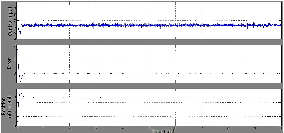
The performance of the overall system is satisfactory while considering linear approximated model of the system in simulations as shown in Table 2. Fig. 6 shows the performance of the controller in real time and the typical values of parameters, obtained through one of the performed trials, are;
Controller Parameters: Kp=1.9, Ki=0.0395, Kd=19.7
Range for good operation: [0.67 to 4.10] cms
Range for optimum operation (error in 2% band): [1.0 to 3.3] cms
VI. CONCLUSION
A brief overview on MIT rule and Differential Evolution soft computing algorithm has been carried out in this paper along with the mathematical modeling of magnetic levitation system. In later sections, closed loop controllers have been designed based on two techniques and the performance of these controllers evaluated in simulations as well as in real time on magnetic levitation system. From the results, one can conclude that the performance of DE based offline tuned PID controller is better than the MIT rule based controller.DE algorithm is very simple and effective search algorithm which takes very less computation time than other soft computing algorithms. The performance of DE based controller with appropriately chosen range for parameters is better than MIT based controller in real time also. Selection of this range is very critical in DE algorithm and is carried out carefully.
The performance of MIT controller is very much depends upon the value of adaptation gain and selection of this gain decides the performance of the system. The drawbacks of DE based controller is that it cannot be applied on systems in real time directly, one has to run few trials first in simulations to generate appropriate values of parameters and the effectiveness of these generated values depends upon the efficient programming carried out by an expert. With large number of parameters in any system, the program may become complex and time consuming.
Figure 6. Simulation diagram of DE based control based magnetic levitation system in real time
REFERENCES
[1] K. J. Astrom and B. Wittenmark, Adaptive Control,2nd ed. New York: Dover Publications Inc., 1995, ch. 5, pp. 185-234.
[2] P. Swarnkar, S. K. Jain, and R. K. Nema, “Effect of adaptation gain on system performance for model reference adaptive control scheme using MIT rule,” presented at International Conference of World Academy of Science, Engineering and Technology, Paris, 2010.
[3] P. Swarnkar, S. Jain, and R. K. Nema, “Application of model reference adaptive control scheme to second order system using MIT rule,” presented at International Conference on Electrical Power and Energy Systems (ICEPES-2010), MANIT, Bhopal, India, 2010.
[4] Priyank Jain and M. J. Nigam, “Real Time Control of Ball and Beam System with Model Reference Adaptive Control Strategy using MIT Rule,” presented at 2013 IEEE International Conference on Computational Intelligence and Computing Research (ICCIC), Madurai, 2013.
[5] R. Storn and K. Price, “Differential evolution-a simple and efficient adaptive scheme for global optimization over continuous spaces,” Journal of Global Optimization, vol. 11, pp. 341-359, 1997.
[6] Rainer Storn. (2005). Differential evolution for continuous function optimization. [Online]. Available: http://www.icsi.berkeley.edu/storn/code.html
[7] K. Price, “An introduction to differential evolution,” in New Ideas in Optimization,D. Corne, M. Dorigo, and F. Glover, Ed. London, UK: McGraw-Hill, 1999, pp. 79-108.
[8] R. Storn, “On the usage of differential evolution for function optimization,” in Proc. IEEE Biennial Conference of the North American Fuzzy Information Processing Society, Berkeley, CA, USA, 1996, PP. 519-523.
[9] M. Valluvan and S. Rangaanathan, “Modeling and control of magnetic levitation system,” in Proc. IEEE International Conference on Emerging Trends in Science, Engineering and Technology, Tiruchirappalli, India, 2012, pp. 545-548.
[10] A.-V. Duka, S. E. Oltean, and M. Dulău, “Model reference adaptive vs. learning control for the inverted pendulum,” presented at the International Conference on Control Engineering and Applied Informatics (CEAI), 2007.
[11] M. S. Ehsani, “Adaptive control of servo motor by MRAC Method,” presented at IEEE International Conference on Vehicle, Power and Propulsion, Arlington, TX, 2007.
[12] K. S. Narendra and A. M. Annaswamy, Stable Adaptive Systems, New Jersey: Prentice-Hall, Englewood Cliffs, 1989.
[13] M. S. Saad, H. Jamaluddin, and I. Z. M. Darus, “PID controller tuning using evolutionary algorithms,” WSEAS Transactions on System and Control,vol. 7, pp. 139-149, 2012.
[14] K. J. Astrom and T. Hagglund, “Automatic tuning of PID controllers,” Research Triangle Park, NC: Instrument Society of America, 1988.
[15] J. G. Ziegler and N. B. Nichols, “Optimum settings for automatic controllers,” Trans. ASME. vol. 64, pp. 759-768, 1942.
Priyank Jain received the B.E. degree in
Electronics and Instrumentation Engineering from S.G.S. Institute of Technology and Science, Indore, India, in 2012. He is currently an M.Tech. student in Department of Electronics and Communication Engineering with specialization in System Modeling and Control, Indian Institute of Technology (IIT) Roorkee, Roorkee, India. His main areas of research interest are linear control systems, adaptive control systems and soft computing techniques.
M. J. Nigam received the B.Tech. degree in