Inzinerine Ekonomika-Engineering Economics, 2011, 22(2), 126-133
Credit Risk Estimation Model Development Process: Main Steps and Model
Improvement
Ricardas Mileris, Vytautas Boguslauskas
Kaunas University of Technology
K. Donelaicio str. 73, LT-44309, Kaunas, Lithuania
e-mail: [email protected], [email protected]
The attribution of credit ratings for clients is a very important issue in the banking sector. Banks must evaluate credit risk of credit applicants by using standardized (external rating institutions) or internal ratings-based (IRB) methods. Banks which decided to use IRB method attempt to develop precise internal credit rating models for the evaluation of creditworthiness of their borrowers.
The internal rating method for the estimation of default probability requires to collect the default information from the historical data in banks. The major studies about default determinating factors are based on classification methods (Zhou, Xie, Yuan, 2008). A classification model considers the default measurement as the pattern recognition where all borrowers are divided to non-default and default groups based on their financial and non financial data. Banks attempt to construct an evaluation model that can be used to discriminate new sample.
This research focuses on a credit rating model development which could attribute credit ratings for Lithuanian companies. The steps of a model’s development and improvement process are described in this paper.
The model’s development begins with the selection of initial variables (financial ratios) characterizing default and non-default companies. 20 financial ratios of 5 years were calculated according to annual financial reports. Then statistical and artificial intelligence methods were selected for the classification of companies into two groups: default and non-default. A discriminant analysis, logistic regression and artificial neural networks (multilayer perceptron) were applied for this purpose. Often statistical methods are not able to operate with a large amount of data, so the analysis of variance, Kolmogorov-Smirnov test and factor analysis were applied for data reduction. Artificial neural networks often are able to analyze a large amount of data so variable selection was accomplished by the network itself calculating ranks of importance for every initial variable. There were constructed 15 classification models and their classification accuracy was measured by calculating correct classification rates. The most accurate was a logistic regression model analyzing data of 3 years (97% of correctly classified companies). Then the sample of companies was supplemented with new data and changes in classification accuracy were estimated. The significant decrease of classification accuracy conditioned the need of model update. For this reason the logistic regression coefficients were recalculated. In order to classify non-default companies into 7 classes: profitability, liquidity, financial structure and individual possibility of default
estimated by a logistic regression model were determined as rating criterions. Then the rating scale was constructed and credit ratings were attributed for companies in the sample. The calculated probabilities of default indicated that some lower ratings have lower probabilities of default. These imperfections were corrected by the modification of a rating scale. The research has shown that the developed model is a valid tool for the estimation of credit risk.
Keywords: bank, credit ratings, credit risk, classification methods.
Introduction
Banking activity is exposed to various risks. Understanding and quantifying these risks is crucial for bank management as well as for stability of the whole economy (Sieczka, Holyst, 2009). Banks tend to lend to firms with high credit quality and not to lend to low credit quality firms. So the most important factor in determining lending practices is credit risk (Daniels, Ramirez, 2008). According to Duff & Einig (2009), research considering credit risk has been one of the most active areas of recent financial research, with significant efforts deployed to analyse the meaning, role, and influence of credit ratings.
The development of the credit rating prediction models has attracted lots of research interests in academic and business community. Many researchers have attempted to construct automatic classification systems using methods from data mining, such as statistical and artificial intelligence techniques (Huang, 2009). These techniques include discriminant analysis (Min, Lee, 2008), logistic regression (Psillaki, Tsolas, Margaritis, 2010), k-nearest neighbour (Twala, 2010), decision trees (Paleologo, Elisseeff, Antonini, 2010), artificial neural networks (Angelini, Tollo, Roli, 2008; Yu, Wang, Lai, 2008), support vector machine (Danenas, Garsva, 2009; Lee, 2007), nearest subspace method (Zhou, Jiang, Shi, 2010), hybrid models (Lin, 2009), etc.
Mostly the scientific publications about estimation of credit risk present models which classify companies into 2 groups: default or non-default. This research is intended for the development of credit risk estimation model which could classify reliable companies into seven classes and not reliable companies into one class.
The object of this research is credit risk estimation models.
The aim of this research is to develop credit risk estimation model and to describe the development process.
The methods of this research:
1. Analysis of scientific publications.
2. Development of a credit risk estimation model. The developed model will allow the bank to estimate the credit risk of Lithuanian companies.
Internal credit rating models in banks
The activity of business companies is directly or indirectly influenced by various internal and external factors (Boguslauskas, Adlyte, 2010). Unfavourable business environment, unexpected and unfavourable events, the risky decisions of enterprise managers may make any enterprise insolvent and lead it towards bankruptcy (Purvinis, Sukys, Virbickaite, 2005). Difficult business environment stimulates to look for new ways to assess the changing situation as well as to implement and manage new means for business continuity (Valackiene, 2010). These negative factors and ability to manage them also influence the credit risk of companies which must be measured by banks properly.
With the rapid growth in credit industry and the management of large loan portfolios, internal credit rating models have been extensively used for the credit admission evaluation. In general, the bank’s internal measures of credit risk are based on assessments of borrower and transaction risk. Mostly banks base their rating methodology on borrower‘s default risk and typically assign a borrower to a credit rating grade (Butera, Faff, 2006). The credit rating models are developed to classify loan applicants as either a reliable group (accepted) or not reliable group (rejected) with their related characteristics based on the data of the previous accepted and rejected applicants (Tsai, Chen, 2010).
The guidelines for measuring credit risk are suggested in the Basel II Capital Accord (Weißbach, Tschiersch, Lawrenz, 2009). With the implementation of the Basel II Capital Accord in 2006, banks are now also allowed to use internal data and rating models for the purpose of estimating own default probabilities (PD) and calculating regulatory capital (Ryser, Denzler, 2009). According to the Basel Committee on Banking Supervision banks are required to measure the one year default probability. So usually statistical credit risk estimation models try to predict the probability that a loan applicant or existing borrower will default in one year (Fantazzini, Figini, 2009). In addition, banks should also provide the loss given default (LGD) – a measure of how much per unit of exposure bank will lose if the client defaults (Butera, Faff, 2006). Credit rating models allow to rate clients credibility and to evaluate expected losses of bank (Sieczka, Holyst, 2009).
One of the central ideas of IRB method that banks are free to choose their own method when:
1. A meaningful differentiation of risk between classes is achieved.
2. Plausible, intuitive, and current input data are used. 3. All relevant information is taken into account
(Ryser, Denzler, 2009).
Commercial banks can use statistical tools to discriminate between reliable and not reliable borrowers and
to measure the credit quality according to internal rating scales (Ryser, Denzler, 2009). There are several well-known statistical techniques for constructing credit rating predictions. These techniques include logistic regression, discriminant analysis, linear probit model, etc. (Hwang, Chung, Chu, 2010). Also methods of artificial intelligence are widely used for classification of companies. In addition, the hybridization approach has been an active research area to improve the classification (prediction) performance over single learning approaches. In general, it is based on combining two different machine learning techniques. Therefore, to develop a hybrid learning credit model, there are three different ways to combine the two machine learning techniques:
1. Combining two classification techniques. 2. Combining two clustering techniques.
3. One clustering technique combined with one classification technique (Tsai, Chen, 2010). These statistical and machine learning techniques analyze the particular data set about credit applicants. So in credit risk estimation model development the successful selection of informative variables is very important. According to Arslan & Karan (2009), different factors affect credit risks of firms. Jiao, Syau & Lee (2007) maintained that the data can be classified into three categories:
1. Financial conditions: liquidity, financial structure, profitability and efficiency ratios.
2. Management measures: administrator’s management experiences, stockholders structure type, conditions of capital increment during the last years, etc. 3. Characteristics and perspectives of products and
competitions: equipment and technologies, product marketability, collateral, economic conditions of the industry in the next year.
Thus, the total credit rating can be obtained by summarizing these three categories. It should be noted that only the first category (financial conditions) can be expressed numerically. Most of the quantities in the other two categories cannot be expressed numerically easily. To overcome this difficulty, fuzzy numbers can be used for linguistic expressions (Jiao, Syau, Lee, 2007).
The interaction between different risk factors and credit ratings was analyzed in many publications. The importance of financial factors is widely accepted because its impact is measurable. The relevance of non-financial factors is mainly considered as not decisive (Grunert, Norden, Weber, 2005). So companies should seek to present a true and fair view of their financial performance and results because banks need informative and truthful accounting data for making right decisions (Rudzioniene, 2006).
The results of a credit risk estimation are credit ratings. Usually credit ratings range from AAA to D. Basing on the rating scale of Standard & Poor‘s, it is possible to group ratings into three categories:
• AAA, AA, A as category 1.
• BBB as category 2.
• Below BBB as category 3.
have adequate capacity to meet their financial commitments. However, firms receiving ratings below BBB mean that they are regarded as having speculative characteristics (Hwang, Chung, Chu, 2010).
The internal rating models have many benefits for banks. These benefits include reducing the cost of credit analysis, enabling faster decisions, ensuring credit collections, and diminishing possible risks. Even a slight improvement in credit rating accuracy may reduce large credit risks and translate into significant future savings (Tsai, Chen, 2010). In addition Ince & Aktan (2009) affirm that credit rating models, used to model the potential risk of loan applications, may be an effective substitute for the use of judgment among inexperienced loan officers, thus helping to control bad debt losses.
When the credit risk estimation model is developed, it is important to evaluate its quality. The low-quality rating models have two important negative effects on a bank’s financial stability. First, return on the portfolio will be lower than expected. If a borrower receives too favorable rating, he will most likely accept the loan offer, whereas rejection is more likely in the case of a rating error in the opposite direction, i.e., the bank will earn money from adverse selection. Second, due to the adverse selection effect, the calculated regulatory capital held by the bank is too low. As more borrowers with too favorable ratings are in the portfolio, the resulting regulatory capital based on these ratings may be inadequate (Hornik, Jankowitsch, Lingo, Pichler, Winkler, 2010).
Credit risk estimation model development
The model for rating of Lithuanian companies was developed in order to measure their credit risk. The main steps of a model‘s development process are described below.
1. Variable selection. For typical classification problems, values for a set of independent variables are given in a set of (training) examples, upon which a model is developed to categorize future observations into appropriate classes (Piramuthu, 2006). In this case the analyst must have the set of variables which allow to estimate the credit risk of companies successfuly. Developing the credit risk estimation model, the set of initial variables consisted of 20 financial ratios of 5 years. So there were 100 independent variables Xi and one dependent variable Y (default or non-default).
2. Data analysis methods selection. Discriminant analysis (DA), logistic regression (LR) and artificial neural networks (ANN) methods were applied for classification of companies into 2 groups: default and non-default.
Discriminant analysis is a commonly used technique to classify a set of observations into predefined classes in various fields (Huang, Kao, Wang, 2007). It is a classification method that can predict the group membership of a newly sampled observation. In DA, a group of observations whose memberships are already identified are used for the estimation of weights in a discriminant function. A new sample is classified into one of several groups by DA results (Sueyoshi, 2006). The goal of linear DA is to find a linear transformation that
maximizes class separability in the reduced dimensional space (Park, Park, 2008). The mathematical model is:
∑
= += n
i i i
x z
1
β
α (1)
where α is an intercept, xiis the value of independent variable,βiis the coefficient of the variable xi.
Two discriminant functions were constructed for default (z1) and non-default (z0) companies in every developed DA model. The company was numbered into group which z gets higher value.
Logistic regression models allow to estimate the indivudual possibility of default for every company in the range of [0; 1]. In a logistic regression model the possibility of individual to default is expressed as follows:
⎟⎟⎠ ⎞ ⎜⎜⎝ ⎛ + + ⎟⎟⎠ ⎞ ⎜⎜⎝ ⎛ + =
∑
∑
= = ni i i
n
i i i
n x x P 1 1 exp 1 exp β α β α (2)
where α is an intercept, xiis the value of independent variable,βiis the coefficient of the variable xi (Dong, Lai, Yen, 2010). The classification threshold of Pn in developed LR models was set to 0.5.
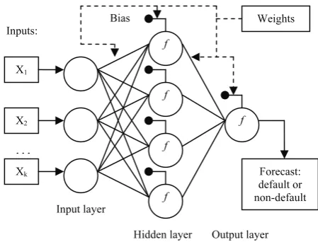
A multilayer perceptron was used for the classification of companies as one of the possible types of ANN (Figure 1).
Figure 1. Multilayer perceptron
In this network, the information flows forward to the output continuously without any feedback (Boguslauskas, Mileris, 2009). The initial variables are fed into input nodes, while the output provides the forecast for the future value. Hidden nodes with appropriate nonlinear transfer functions are used to process the information received by the input nodes. The model can be written as:
t m
j
n
i ij i j j
t f x
y α α β β +ε
⎟⎟⎠ ⎞ ⎜⎜⎝ ⎛ + + =
∑
∑
=1 =1 0
0 (3)
where n is the number of input nodes, m is the number of hidden nodes, f is a sigmoid transfer function, {αj, j = 0, 1, ..., m} is a vector of weights from the hidden to output
f f f f f
…
X1 X2 Xk Bias Forecast: default or non-default Weights Inputs: Input layernodes, {βij, i = 1, 2, ..., n; j = 0, 1, ..., m} are weights from the input to hidden nodes, α0 and β0j are weights of connections leading from the bias which have values always equal to 1 (Azadeh, Ghaderi, Sohrabkhani, 2007).
3. Data reduction. Not all initial variables are useful for the analysis, so it is important to find informative parameters for credit risk estimation model development in the set of initial variables. Also the statistical methods often are not able to analyze high amount of data, so the need of data reduction arises. Four methods for data reduction were applied: the analysis of variance (ANOVA), Kolmogorov-Smirnov test (K-S), factor analysis (FA) and ranks of importance in ANN (ROI).
Figure 2 illustrates the process of data reduction for classification models. The 1st column consists of the period of data (from the last year to 5 years ago) and number of initial variables. The 2nd and 3rd columns show methods applied for data reduction. In the 4th column there is a number of variables used for classification of companies. The 5th column consists of a code of classification models (method and period of data analyzed).
Figure 2. Data reduction for classification models
The purpose of ANOVA is to test for significant differences between means of independent variables in groups of failed and not failed companies. If the means did not differ significantly the variable was rejected from further analysis.
The Kolmogorov-Smirnov one sample test for normality is based on the maximum difference between the sample cumulative distribution and the hypothesized cumulative distribution (Mileris, Boguslauskas, 2010). This test allowed to verify if the variable has the normal distribution. If the statistics D of K-S test is significant, then the hypothesis that the respective distribution is
normal should be rejected. These variables were not included into the credit risk analysis.
Factor analysis is a statistical method that is based on the correlation analysis of variables. The purpose is to reduce multiple variables to a lesser number of factors (Ocal, Oral, Erdis, Vural, 2007). The reduction of observed initial variables to less factors allows to enhance interpretability and detect hidden structures in the data (Treiblmaier, Filzmoser, 2010).
These methods were applied for data reduction before DA and LR models were developed. Artificial neural networks are able to operate with a large amount of data, so all initial variables were fed to them. Ranks of importance were attributed for every variable by ANN itself. The variables that ROI > 0 were included into further analysis.
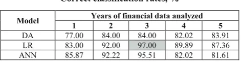
4. Estimation of classification accuracy. Overall 15 models were developed for the classification of companies into 2 groups. The correct classification rates (CCR) were calculated for the estimation of classification accuracy (Table 1). These rates indicate the proportion of correctly classified companies by a certain model.
Table 1
Correct classification rates, %
Model Years of financial data analyzed
1 2 3 4 5
DA 77.00 84.00 84.00 82.02 83.91 LR 83.00 92.00 97.00 89.89 87.36 ANN 85.87 92.22 95.51 82.02 81.61
The highest classification accuracy (97%) was reached by the logistic regression model which employed three-years financial data of companies. So this LR3 model was used for the estimation of credit risk.
5. Estimation of changes in classification accuracy.
The classification model LR3 was developed using financial ratios of 2004-2006 years. The data of 100 Lithuanaian companies was analyzed. After that the initial data set was complemented with financial ratios of 2006-2008 years of 100 new companies and the changes in classification accuracy were estimated. The test of model indicated that the correct classification rate decreased to 82.23% (Table 2). It is the significant decrease (Δ1 = -14.77%) so the need of model update arised.
6. Update of classification model. The regression coefficients were recalculated for the same 25 variables of LR3 model. The CCR of updated classification model increased to 93.43% (Table 2). The increase influenced on model update was 11.2% (Δ2).
Table 2
Changes of CCR
LR3 Test Δ1 Updated Δ2
97.00 82.23 -14.77 93.43 +11.2
Changes of CCR show the importance of model update when bank gets new data about clients. The update can significantly improve the classification model‘s performance.
7. Determination of ratings criterions. The factor analysis has shown that 3 factors which explain 40.4% – 1 year
(X1-X20)
2 years (X1-X40)
3 years (X1-X60)
4 years (X1-X80)
5 years (X1-X100)
ANOVA
ANOVA
ROI
ANOVA
ANOVA
ROI
ANOVA
ANOVA
ROI
FA
FA
ROI
FA
FA
ROI
9
K-S 6 DA1
LR1
15 ANN1
K-S 11 DA2
16 LR2
37 ANN2
K-S 12 DA3
25 LR3
50 ANN3
17
17
73
20
17
86
DA4
LR4
ANN4
DA5
LR5
42.8% of total variance are: profitability, liquidity and financial structure. So from an initial set of variables 4 profitability, 2 liquidity and 1 financial structure ratios were selected which had the highest correlation coefficients |r| with individual possibility of default (Pn).
Table 3
Correlation coefficients between financial ratios and Pn
Group Financial ratio r |r|
Profitability: NPM -0.27147 0.27147
EBIT/TA -0.50944 0.50944
NP/TA -0.48495 0.48495
EBIT/S -0.31458 0.31458
Liquidity: CR -0.15071 0.15071
QR -0.12926 0.12926
Financial structure: DR 0.181803 0.181803
In Table 3 NPM is a net profit margin, EBIT/TA is earnings before interest and taxes to total assets, NP/TA is net profit to total assets, EBIT/S is earnings before interest and taxes to sales, CR is current ratio, QR is quick ratio, DR is debt ratio. As a criterion of ratings the individual possibility of default also included into analysis. So the profitability determines 50%, liquidity – 25%, financial structure – 12.5%, individual possibility of default – 12.5% of credit rating.
8. Construction of rating scale. The rating model is based on classification of companies according to logistic regression analysis results and rating criterions (Figure 3).
Figure 3. Attribution of credit ratings
The variables Xi were analyzed by the logistic regression (LR3) model. According to estimated individual possibility of default (Pn), companies were classified into 2 classes: default and non-default. For companies classified by LR3 model as default the rating D1 was attributed. The Basel II Capital Accord requires that non-default companies must be classified at least into 7 classes. So according to the determined rating criterions ratings AAA – C were attributed for reliable companies. In addition, if company by LR3 model was classified as reliable but its financial ratios are bad, for such companies rating D2 was attributed.
In group of not default companies 5 statistical characteristics were calculated for 7 financial ratios: minimum value (Min), maximum value (Max), standard deviation (σ), mean (μ) and median (Me). The exceptions (E) of values were rejected from further analysis:
E ∉ (μ - 3σ; μ + 3σ) (4)
Then Min, Max and Me values in the sample were recalculated. In order to create rating scale the interval of values for each financial ratio was divided into 2 sections:
• Min – Me (from minimum to median).
• Me – Max (fom median to maximum).
Every section was divided into 4 equal intervals and the margins of financial ratios in these intervals were calculated. According to the values of financial ratios and individual possibility of default (Pn), scores were attributed for companies (Table 4).
Table 4
Intervals of rating criterions and scores
Score NPM EBIT/TA ... Pn 7 > 0.75 > 0.38 ... ≤ 0.001 6 (0.51; 0.75] (0.28; 0.38] ... (0.001; 0.003]
... ... ... ... ...
0 ≤ 0.01 ≤ -0.0772 ... > 0.541
The credit rating of a company depends on the sum of scores (Table 5).
Table 5
Credit ratings and total scores
Rating AAA AA A ... D2
Total score 50-56 43-49 36-42 ... 0-7
9. Calculation of probabilities of default. The probabilities of default (PD) were calculated for every rating:
% 100
× =
C C I N
PD (5)
where NC – number of default companies in particular rating, IC - number of companies in particular rating.
The probabilities of default illustrated in Figure 4.
100 91.1
14.3 8.3 1.9 6.1 3.8 0 -0 20 40 60 80 100 120
AAA AA A BBB BB B C D1 D2
%
Figure 4. Probabilities of default (%) and credit ratings
Grunert, Norden & Weber (2005) point out the necessity of a link between credit rating and probability of default. The credit rating models of high quality have the inverse relation between credit ratings and PD values: when the credit ratings decrease the PD values constantly increase. In developed model ratings A and BBB have higher PD than rating BB. Also it was impossible to calculate PD for rating AAA because no one company got this rating. So it is worth to modify the rating scale in order to improve the model‘s performance.
X1
LR3
Non-default Pn∈ [0; 0.5)
Default Pn∈ [0.5; 1]
Rating criterions X2
…
Xn
AAA
AA
A
BBB
BB
B
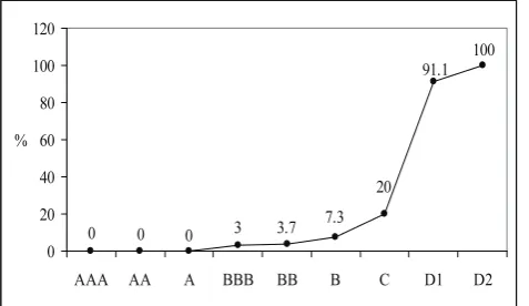
C
10. Modification of rating scale. The intervals of total scores were changed (Table 5) and all imperfections were corrected (Figure 5).
100 91.1
20 7.3 3.7 3 0 0 0 0 20 40 60 80 100 120
AAA AA A BBB BB B C D1 D2
%
Figure 5. PD (%) and credit ratings of modified scale
Companies with ratings D1 and D2 can be considered as one class of not reliable clients and bank should not credit them. These ratings can be merged to one rating D.
The probability of default of companies with ratings AAA, AA and A is equal to 0. The difference between these ratings is influenced on the financial state of companies. The companies with higher ratings have higher average profitability and liquidity ratios. Also these companies have lower average debt ratio and individual
possibility of default. So according to the rating of reliable companies, a bank can determine the interest rate for loans.
Conclusions
1. This research confirmed that the discriminant analysis, logistic regression and artificial neural networks are relevant methods for the classification of banks clients. The highest classification accuracy (97%) was reached by the logistic regression model.
2. The analysis of variance, Kolmogorov-Smirnov test and factor analysis are statistical methods capable to reduce a large amount of data and help to select variables for the estimation of credit risk.
3. The percentage of credit rating criterions suggested in this research is: profitability – 50%, liquidity – 25%, leverage – 12.5%, individual possibility of default estimated by logistic regression – 12.5%. These criterions allowed to create valid rating scale for the measurement of Lithuanian companies credit risk. 4. The recalculation of classification functions
coefficients when new data of clients available can improve the correct classification results of the model. Also the changing of total scores intervals can improve a model‘s rating scale.
5. The described steps of the credit risk estimation model development can help other researchers to create models which allow to measure credit risk successfuly.
References
Angelini, E., Tollo, G., & Roli, A. (2008). A Neural Network Approach for Credit Risk Evaluation. The Quarterly Review of Economics and Finance, 48(4), 733-755.
Arslan, O., & Karan, M. B. (2009). Credit Risks and Internationalization of SMEs. Journal of Business Economics and Management, 10(4), 361-368.
Azadeh, A., Ghaderi, S. F., & Sohrabkhani, S. (2007). Forecasting Electrical Consumption by Integration of Neural Network, Time Series and ANOVA. Applied Mathematics and Computation, 186(2), 1753-1761.
Boguslauskas, V., & Adlyte, R. (2010). Evaluation of Criteria for the Classification of Enterprises. Inzinerine Ekonomika-Engineering Economics, 21(2),119-127.
Boguslauskas, V., & Mileris, R. (2009). Estimation of Credit Risk by Artificial Neural Networks Models. Inzinerine Ekonomika-Engineering Economics(4),7-14.
Butera, G., & Faff, R. (2006). An Integrated Multi-Model Credit Rating System for Private Firms. Review of Quantitative Finance and Accounting, 27(3), 311-340.
Danenas, P., & Garsva, G. (2009). Support Vector Machines and their Application in Credit Risk Evaluation Process.
Transformations in Business & Economics, 3(18), 46-58.
Daniels, K., & Ramirez, G. G. (2008). Information, Credit Risk, Lender Specialization and Loan Pricing: Evidence from the DIP Financing Market. Journal of Financial Services Research, 34(1), 35-59.
Dong, G., Lai, K. K., & Yen, J. (2010). Credit Scorecard Based on Logistic Regression with Random Coefficients.
Procedia Computer Science, 1(1), 2457-2462.
Duff, A., & Einig, S. (2009). Understanding Credit Ratings Quality: Evidence from UK Debt Market Participants. The British Accounting Review, 41(2), 107-119.
Fantazzini, D., & Figini, S. (2009). Random Survival Forests Models for SME Credit Risk Measurement. Methodology and Computing in Applied Probability, 11(1), 29-45.
Grunert, J., Norden, L., & Weber, M. (2005). The Role of Non-Financial Factors in Internal Credit Ratings. Journal of Banking & Finance, 29(2), 509-531.
Huang, Y., Kao, T. L., & Wang, T. H. (2007). Influence Functions and Local Influence in Linear Discriminant Analysis.
Computational Statistics & Data Analysis, 51(8), 3844-3861.
Huang, S. C. (2009). Integrating Nonlinear Graph Based Dimensionality Reduction Schemes with SVMs for Credit Rating Forecasting. Expert Systems with Applications, 36(4), 7515-7518.
Hwang, R. C., Chung, H., & Chu, C. K. (2010). Predicting Issuer Credit Ratings Using a Semiparametric Method. Journal of Empirical Finance, 17(1), 120-137.
Ince, H., & Aktan, B. (2009). A Comparison of Data Mining Techniques for Credit Scoring in Banking: A Managerial Perspective. Journal of Business Economics and Management, 10(3), 233-240.
Jiao, Y., Syau, Y. R., & Lee, E. S. (2007). Modelling Credit Rating by Fuzzy Adaptive Network. Mathematical and Computer Modelling, 45(5-6), 717-731.
Lee, Y. C. (2007). Application of Support Vector Machines to Corporate Credit Rating Prediction. Expert Systems with Applications, 33(1), 67-74.
Lin, S. L. (2009). A New Two-Stage Hybrid Approach of Credit Risk in Banking Industry. Expert Systems with Applications, 36(4), 8333-8341.
Mileris, R., & Boguslauskas, V. (2010). Data Reduction Influence on the Accuracy of Credit Risk Estimation Models.
Inzinerine Ekonomika-Engineering Economics, 21(1),5-11.
Min, J. H., & Lee, Y. C. (2008). A Practical Approach to Credit Scoring. Expert Systems with Applications, 35(4), 1762-1770.
Ocal, M. E., Oral, E. L., Erdis, E., & Vural, G. (2007). Industry Financial Ratios – Application of Factor Analysis in Turkish Construction Industry. Building and Environment, 42(1), 385-392.
Paleologo, G., Elisseeff, A., & Antonini, G. (2010). Subagging for Credit Scoring Models. European Journal of Operational Research, 201(2), 490-499.
Park, C. H., & Park, H. (2008). A Comparison of Generalized Linear Discriminant Analysis Algorithms. Pattern Recognition, 41(3), 1083-1097.
Piramuthu, S. (2006). On Preprocessing Data for Financial Credit Risk Evaluation. Expert Systems with Applications, 30(3), 489-497.
Psillaki, M., Tsolas, I. E., & Margaritis, D. (2010). Evaluation of Credit Risk Based on Firm Performance. European Journal of Operational Research, 201(3), 873-881.
Purvinis, O., Sukys, P., & Virbickaite, R. (2005). Research of Possibility of Bankruptcy Diagnostics Applying Neural Network. Inzinerine Ekonomika-Engineering Economics(1),16-22.
Rudzioniene, K. (2006). Impact of Stakeholders’ Interests on Financial Accounting Policy-Making: The Case of Lithuania.
Transformations in Business & Economics, 1(9), 51-64.
Ryser, M., & Denzler, S. (2009). Selecting Credit Rating Models: A Cross-Validation-Based Comparison of Discriminatory Power. Financial Markets and Portfolio Management, 23(2), 187-203.
Sieczka, P., & Holyst, J. A. (2009). Collective Firm Bankruptcies and Phase Transition in Rating Dynamics. The European Physical Journal B - Condensed Matter and Complex Systems, 71(4), 461-466.
Sueyoshi, T. (2006). DEA-Discriminant Analysis: Methodological Comparison Among Eight Discriminant Analysis Approaches. European Journal of Operational Research, 169(1), 247-272.
Treiblmaier, H., & Filzmoser, P. (2010). Exploratory Factor Analysis Revisited: How Robust Methods Support the Detection of Hidden Multivariate Data Structures in IS Research. Information & Management, 47(4), 197-207.
Tsai, C. F., & Chen, M. L. (2010). Credit Rating by Hybrid Machine Learning Techniques. Applied Soft Computing, 10(2), 374-380.
Twala, B. (2010). Multiple Classifier Application to Credit Risk Assessment. Expert Systems with Applications, 37(4), 3326-3336.
Valackiene, A. (2010). Efficient Corporate Communication: Decisions in Crisis Management. Inzinerine Ekonomika-Engineering Economics, 21(1),99-110.
Weißbach, R., Tschiersch, P. & Lawrenz, C. (2009). Testing Time-Homogeneity of Rating Transitions After Origination of Debt. Empirical Economics, 36(3), 575-596.
Yu, L., Wang, S., & Lai, K. K. (2008). Credit Risk Assessment with a Multistage Neural Network Ensemble Learning Approach. Expert Systems with Applications, 34(2), 1434-1444.
Zhou, X., Jiang, W., & Shi, Y. (2010). Credit Risk Evaluation by Using Nearest Subspace Method. Procedia Computer Science, 1(1), 2443-2449.
Ričardas Mileris, Vytautas Boguslauskas
Kredito rizikos vertinimo modelio sudarymo procesas: pagrindiniai etapai ir modelio tobulinimas
Santrauka
Kredito rizikos vertinimas yra vienas iš kredito suteikimo etapų. Pagrindinis kredito rizikos vertinimo tikslas yra nustatyti, ar verta suteikti kreditą. Bankai stengiasi sumažinti kredito riziką, nesuteikdami kreditų klientams, kurie turi mažiausias galimybes įvykdyti prisiimtus finansinius įsipareigojimus. Suteikus kreditą, skolininko kredito rizikos lygis taip pat būtinas banko kapitalo pakankamumui apskaičiuoti.
Vienas iš kredito rizikos vertinimo būdų yra bankų vidaus kredito rizikos vertinimo modelių taikymas. Šiuos modelius bankai sudaro atsižvelgdami į savo poreikius ir turimus duomenis, pasirenka tinkamiausius duomenų analizės metodus. Mokslinėse publikacijose dažniausiai aprašomi modeliai, kuriais įmonės klasifikuojamos į 2 grupes (patikimų ir nepatikimų klientų). Bazelio bankų priežiūros komiteto rekomendacijose nurodyta, kad patikimos įmonės turi būti suskirstytos į ne mažiau kaip 7 grupes (reitingus). Todėl šiame tyrime buvo siekiama sudaryti įmonių kredito rizikos vertinimo modelį, kuriuo patikimi banko klientai klasifikuojami į 7 grupes, o nepatikimi – į 1 grupę.
Šio tyrimo objektas – įmonių kredito rizikos vertinimo modeliai.
Tyrimo tikslas – sudaryti įmonių kredito rizikos vertinimo modelį ir aprašyti jo sudarymo proceso etapus. Tyrimo metodai:
• Mokslinių publikacijų, susijusių su kredito rizikos vertinimu, analizė.
• Įmonių kredito rizikos vertinimo modelio sudarymas.
Įmonių aplinkos pokyčiai daro įtaką jų patikimumui kredito rizikos atžvilgiu ir keičia patikimumo vertinimo kriterijus. Todėl, atsižvelgiant į šiuos pokyčius, aktualu nuolat atnaujinti bankų taikomus klientų kredito rizikos vertinimo modelius. Tyrime buvo siekiama sudaryti modelį, kuriuo bankas galėtų kiekybiškai įvertinti įmonių kredito riziką. Taigi šiame straipsnyje aprašyta modelio esmė ir jo sudarymo proceso etapai.
Modelio sudarymas pradėtas kintamųjų rinkinio formavimu. Buvo suskaičiuota 20 santykinių finansinių rodiklių, kurie apima 5 metų įmonių veiklos rezultatus, t. y. buvo sudarytas pradinių 100 kintamųjų rinkinys. Toliau pasirinkti duomenų analizės metodai, kuriais galima klasifikuoti įmones į patikimų ir nepatikimų įmonių grupes: diskriminantinė analizė, logistinė regresija ir dirbtinių neuronų tinklai (DNT). Diskriminantinės analizės metodu įmonėms klasifikuoti į patikimų ir nepatikimų klientų grupes buvo sudarytos 2 klasifikavimo funkcijos. Klasifikuojant tiriamoji įmonė priskiriama tai grupei, kurios klasifikavimo funkcija įgyja didesnę reikšmę. Logistinės regresijos metodu įmonių klasifikavimo modelį galima sudaryti taip, kad būtų prognozuojamas ne dichotominis, o tolydusis kintamasis, kurio reikšmių intervalas yra [0; 1]. Šiuo atveju nustatoma galimybė, kad įmonė neįvykdys prisiimtų finansinių įsipareigojimų bankui. Apskaičiuotos reikšmės įvertina įmonės individualią finansinių įsipareigojimų neįvykdymo galimybę nuo 0 iki 100 proc. Nustatyta įmonių klasifikavimo slenksčio reikšmė – 0,5. Trečiasis metodas, kuriuo buvo klasifikuojamos įmonės – DNT. Pagrindinis DNT skirtumas, palyginti su statistiniais duomenų analizės metodais, yra tas, kad DNT neturi tikslaus išankstinio duomenų analizės modelio, o sudaro jį patys pagal į tinklą įvestą informaciją. Pasirinktas analizei DNT tipas – daugiasluoksnis perceptronas.
Statistiniai objektų klasifikavimo metodai dažnai negali apdoroti didelio informacijos kiekio. Taip pat į įmonių klasifikavimo procesą nėra tikslinga įtraukti mažai informatyvių parametrų, todėl buvo mažinama pradinio kintamųjų rinkinio apimtis. Duomenų apimčiai sumažinti diskriminantinės analizės ir logistinės regresijos modeliuose pritaikyta vienfaktorinė dispersinė analizė (ANOVA), Kolmogorovo ir Smirnovo kriterijus bei faktorinė analizė. Atliekant vienfaktorinę dispersinę analizę, buvo nustatyta, kurių kintamųjų vidurkiai skirtingų įmonių grupėse statistiškai reikšmingai nesiskiria. Kolmogorovo ir Smirnovo kriterijumi nustatyti požymiai, kurių pasiskirstymas grupėse nėra normalusis. Tokie požymiai nebuvo įtraukti į įmonių klasifikavimą. Faktorinės analizės tikslas – pakeisti požymių, apibūdinančių stebimą reiškinį, rinkinį tam tikru faktorių skaičiumi. Atliekant faktorinę analizę, kintamieji suskirstomi į grupes pagal jų koreliacijas su tam tikrais tiesiogiai nestebimais (latentiniais) faktoriais. Faktorinė analizė leido didelį kiekį kintamųjų paaiškinti išskirtaisiais faktoriais. Taip sumažintas analizuojamų duomenų kiekis, o faktorinės analizės rezultatai įtraukti į analizę kitais daugiamatės statistikos metodais. DNT pasižymi galimybe apdoroti didelius informacijos kiekius, todėl šiems modeliams duomenų apimtis, taikant papildomus statistinius duomenų analizės metodus, nebuvo mažinama. Analizei reikšmingi kintamieji buvo atrinkti pačių neuronų tinklų, atsižvelgiant į kintamųjų reikšmingumo rangus. Įmones suklasifikuoti į dvi grupes buvo sudaryta po 5 diskriminantinės analizės, logistinės regresijos ir DNT modelius. Jie skiriasi analizuojamų duomenų laikotarpiu (nuo 1 iki 5 metų).
Tiksliausio modelio atranka buvo atliekama remiantis teisingo klasifikavimo rodiklio reikšmėmis. Didžiausia šio rodiklio reikšmė pasiekta logistinės regresijos modeliu analizuojant 3 metų įmonių duomenis (LR3 modelis). LR3 modelis buvo sudarytas analizuojant 2004 – 2006 m. Lietuvoje veikiančių ir bankrutavusių 100 įmonių duomenis. Buvo siekiama nustatyti modelio klasifikavimo tikslumo rodiklio pokytį, analizuojant vėlesnių laikotarpių įmonių finansinius rodiklius. Tuo tikslu analizuotų duomenų rinkinys buvo papildytas 2006 – 2008 m. Lietuvoje veikiančių 100 įmonių duomenimis. Teisingo klasifikavimo rodiklis, parodantis bendrą įmonių klasifikavimo tikslumą, sumažėjo 14,77 proc. Šis reikšmingas neigiamas pokytis lėmė modelio atnaujinimo poreikį. Atsižvelgiant į tai, buvo perskaičiuoti LR3 modelio regresijos lygties koeficientai. Tai padidino modelio klasifikavimo tikslumą 11,2 proc.
Reitingai patikimoms įmonėms priskirti remiantis paskutiniojo analizuojamo laikotarpio santykiniais finansiniais rodikliais. Finansinių rodiklių atranka buvo atliekama skaičiuojant porinės koreliacijos koeficientus tarp logistinės regresijos modeliu nustatytos įmonių individualios finansinių įsipareigojimų neįvykdymo galimybės ir santykinių rodiklių reikšmių. Analizei atrinkti labiausiai koreliuojantys rodikliai. Įmonės kredito reitingą lemia: 50 proc. – įmonės pelningumas, 25 proc. – likvidumas, 12,5 proc. – finansų struktūra, 12,5 proc. – individuali įmonės įsipareigojimų neįvykdymo galimybė. Analizuojamų rodiklių reikšmių intervalas buvo padalytas į dvi atkarpas: nuo mažiausios reikšmės iki medianos ir nuo medianos iki didžiausios reikšmės. Kiekviena iš šių atkarpų padalyta į 4 vienodas dalis, suskaičiuotos rodiklių reikšmių ribos. Buvo sudaryti rodiklių reikšmių intervalai ir pagal juos įmonei priskiriamas balas. Pagal įmonės balų sumą įmonei priskiriamas kredito reitingas.
Kiekvieno reitingo grupės įmonėms buvo suskaičiuotos finansinių įsipareigojimų neįvykdymo tikimybės. Mažėjant reitingui kokybiško kredito rizikos vertinimo modelio tikimybės turi būti išsidėsčiusios didėjančiai. Tuo tikslu sudarytas modelis buvo modifikuojamas, t. y. pakeisti balų intervalai, pagal kuriuos priskiriamas reitingas.
Įmonių reitingavimas vykdomas dviem etapais. Įmonės santykiniai finansiniai rodikliai analizuojami atnaujintu logistinės regresijos modeliu. Pagal gautą individualią įmonės finansinių įsipareigojimų neįvykdymo galimybę įmonė klasifikuojama į patikimų arba nepatikimų įmonių grupę. Nepatikimų įmonių grupės įmonėms priskiriamas reitingas D1. Patikimų įmonių grupės įmonės analizuojamos vertinimo balais metodu. Pagal šios analizės rezultatus įmonei priskiriamas kredito reitingas nuo AAA iki D2. Siekiant padidinti modelio veiksmingumą, įmonėms, kurios logistinės regresijos modeliu klasifikuotos kaip patikimos, tačiau vertinimo balais metodu jų rezultatai žemiausi, priskiriamas reitingas D2, reiškiantis įmonės finansinių įsipareigojimų neįvykdymą. Nepatikimos įmonės gali būti klasifikuojamos ir į vieną grupę. Todėl reitingus D1 ir D2 galima sujungti į reitingą D. Tyrimas parodė, kad sudarytas įmonių kredito rizikos vertinimo modelis gali būti veiksminga priemonė Lietuvoje veikiančių įmonių kredito rizikai vertinti.
Raktažodžiai: bankas, kredito reitingai, kredito rizika, klasifikavimo metodai.
The article has been reviewed.