Application of Particle Swarm Optimization in Gain Tuning of Integrated Flight and Propulsion Control

Application of Particle Swarm Optimization in Gain

Tuning of Integrated Flight and Propulsion Control

M. Montazeri-Gh, S. Jafari

*

, M. Nasiri

Systems Simulation and Control Laboratory, Department of M echanical Engineering, Iran University of Science and Technology (IUST)

Abstract

This paper presents the application of partic le swarm optimizat ion for gain tuning of integrated flight and propulsion control. For this purpose, an integrated simu lation of the a irc raft body and the gas turbine engine is first developed. Conventional fuel controlle r for the a ircra ft engine and glide slope and velocity controllers for the aircra ft body are then designed separately based on control require ments and constraints. Subsequently, the gains of the controllers are tuned by particle swarm optimization, where the tuning process is formu lated as an optimization proble m. In th is approach, the pilot lever angle tracking and smooth and stable operation for the engine, as well as the glide angle tracking and the smooth variation of velocity in flight maneuver for the body, are considered as the objective functions to be optimized. Moreover, the effect of neighbor acceleration on optimization results is studied. The results show that the neighbor acceleration factor has a considerable effect on the convergence rate of the particle swarm process. Finally, the results obtained from the simulation of the optimized controlle rs for integrated flight and propulsion control confirm the effectiveness of the proposed approach and its ability to design an optima l controllers resulting in an imp roved flight and propulsion performance wh ile ensuring protection against the physical limitations.

Keywords

Integrated Flight and Propulsion Control, Partic le Swa rm Optimization, Ne ighbor Acceleration Effect

1. Introduction

In the early 1980s, the US Air Force init iated a study called the DM ICS with the objective of developing method ologies for the design of IFPC la ws for an advanced tactical aircra ft[1]. Two very different approaches to IFPC design w ere developed as a result of this study. These methods are a centralized approach, wh ich consists of designing a "global" integrated compensator considering the fully integrated syst em asone high-order system[2], and a decentralized hierarc hical approach, wh ich consists of partit ioning the integrated system into loosely coupled subsystems and then designing separate controllers for the sub-systems such that some high-level performance c riterion is met[3].

Owing to bilatera l e ffects between the aircraft engine and body, separate optimization of propulsion and body might cause suboptimal system perfo rmance. There fore, IFPC p a r ameters should be tuned and optimized simultaneously. One of the co mple xit ies of IFPC design is simultaneous c on t ro ll ers gain tuning. The tradit ional approaches for the tuning of the control parameters, such as manual tuning approaches, are based on tria l a nd e rro r and ma y not resu lt in an optimized engine and body performance. Consequently, the

* Corresponding author: [email protected] (S. Jafari)

Published online at http://journal.sapub.org/aerospace

Copyright © 2013 Scientific & Academic Publishing. All Rights Reserved

tuning process for the controller para meters is viewed as an optimization proble m. Due to the nonlinearity and the switc hing nature of the industrial GTE control strategy[4], as we ll as to comple xity of gain tuning for the flight controller, gra dient - based optimization methods have weak performance for gain tuning. As a result, this proble m requires anon-gradi ent optimization technique. In this study, the PSO is investigated for simultaneous tuning of the IFPC para meters in order to ach ieve an improved performance for the engine and body. In addition, the effect o f neighbor acce leration on PSO results is studied.

illustrated that the use of mixed evaluations by metamodels / CFD can significantly reduce the computational cost of PSO while y ield ing optimal designs as good as those obtained with the costly evaluation tool[15]. Moreover, Bessette and Spencer successfully e mployed the PSO for space trajectoryoptimization[16, 17]. In 2012, Montazeri et.a l used the PSO method for a jet engine M in-Ma x fuel controller design in order to reduce the fuel consumption and response time of a turbojet engine[18].

This paper applies the PSO in the IFPC gain tuning problem for the first time. For this purpose, an integrated flight and propulsion model is firstly developed in order to simu late the bilateral effects between the engine and body. The model consists of a 6 D.O.F nonlinear flight simu lation which is derived fro m the equations of mot ion and aerodyna mic equations, and a turbojet engine Wiener model which is confirmed by e xperimental data. The structure of the GTE fuel controller is then described based on an industrial fuel control strategy. A conventional glide slope control as well as a velocity control is also designed for the flight control system. Subsequently, the simu ltaneous tuning of the IFPC parameters is formulated as an optimizat ion proble m based on the PSO approach. For this optimization proble m, the objective function is defined to min imize the PLA tracking error and oscillation of the operational para meters for the engine as well as the glide slope trac king and s mooth variation of velocity for the body. Moreover, the effect of neighbor acceleration on PSO results is studied. Fina lly, the results of the PSO with and without neighbor acceleration factor are co mpared with the DP and the GA results to investigate the effectiveness of the proposed technique for IFPC gain tuning proble m.

2. Integrated Flight and Propulsion

Simulation

In order to perform the optimizat ion of the a irc raft GTE and body controllers in a practica l manner, it is necessary to simu late these two systems simultaneously. This is because of the bilateral e ffects between the engine and the body in various flight conditions. In other wo rds, separate optimizat ion of the airc raft engine or flight controllers may not satisfy the safe operation of the aircraft in various operating conditi ons. To achieve this purpose, a comb ined dyna mic simu lati on consisting of both engine and flight is needed. In this section, simu ltaneous modeling of the engine and flight simu lator is developed to evaluate the performance of the controllers.

2.1. GTE Modeling

The turbojet is the simplest form of gas turbine in that the hot gases generated in the combustion process escape through an exhaust nozzle to produce thrust. The ma in components of a basic GTE are shown in Figure 1[19].

Figure 1. Schematic of a basic GT E

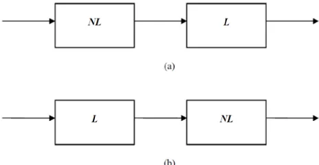
Modeling of a GTE in order to design a controller usually carried out with transfer function or simp lified thermodyna mic models. Also block-structure model is used extensively for this purpose. Block-structured systems are systems that can be represented by interconnections of linear dynamic models and static nonlinear systems. The Ha mmerstein mode l shown in Figure 2 (a ) consists of the cascadeconnecti on of a static nonlinearity follo wed by a linear time-invariant system. Ha mmerstein mode ls are usually used to approxima te systems, where the nonlinearity is caused only by the variation of dc ga in with input a mp litude. These models have constant dynamic behavior regardless of the input a mplitude. It thus seems that Hammerstein models are not appropriate for nonlinear gas turbine modeling since the dynamics of the engine changes with the input amplitude. The Wiener model shown in Figure2 (b) consists of a linear dynamic ele ment in series with a static nonlinear pa rt. Unlike Ha mmerstein models, the nonlinearity in Wiener models is caused by the variation of the system static and dynamic characteristics with input a mplitude. W iener models thus seem to be appro priate candidates for nonlinear gas turbine modeling[20].

Figure 2. Nonlinear model structures: (a) Hammerstein (b) Wiener

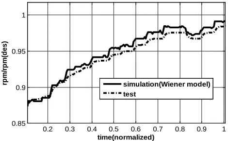
Figure3 co mpares the simulation results with the e xperimental data. The good agreement between the results support the simu lation model used in this study.

0.2 0.3 0.4 0.5 0.6 0.7 0.8 0.9 1

0.85 0.9 0.95 1

time(normalized)

rp

m/

rp

m(

d

e

s

)

simulation(Wiener model) test

Figure 3. Comparison between GTE simulation and experimental results

2.2. Flight Simul ati on

The flight mathematica l mode l used in this study is a nonlinear representation of an aircra ft with rigid body. The rig id body motion is modeled using six nonlinear force and mo ment equations and six kine matics equations. So the aircra ft dyna mics are modeled as a set of 12 first-order coupled nonlinear differentia l equations:

( )

(

( ) ( )

)

( )

(

( ) ( )

)

t =f t , t ,

t =h t , t .

X X u

y X u



(1)

The state vector is defined the same as the output vector and can be represented as:

[

]

= u v w p q r

θψx y z ,

Y

=

X

ϕ

(2)

where:

u, v, w: a ir speed in body axes, p, q, r: body roll, p itch and yaw rates,

θ φ ψ: Euler orientation angles,

x, y, z: Position of the body center of mass, And the control vector is defined as:

[

e r a

]

=δδδf ,

u

(3)

where:

e

a

r

δ : elevator deflection,

δ : aileron deflection,

δ : rudder deflection,

f : engine thrust.

The equations of motion are developed based on the assumption of the flat ea rth and constant mass properties. Also, aerodynamic forces and mo ments are obtained using stability and control derivatives based on an extensive theoretical works given in the format of a nu merica l look-up table.

In this research, the aircra ft maneuver is in the vertical plane. So, the airc raft is ma intained at a constant glide angle

just by trimming the elevator deflection (

δ

_e) provided by the

flight path controller. Moreover, the a irc raft forwa rd speed (u) is controlled by the engine thrust (f) and the elevator

deflection (

δ

_e).

2.3. Integr ation be twee n Flight Simul ation and GTE Model

The methodology used in this study for integration of flight simulat ion and engine model is to simu late the engine and airfra me dyna mics in a modular fashion to test both engine and body controllers for various altitudes, Mach nu mbers and p ilot co mmands. The schematic of the integrated engine and airfra me simu lation is shown in Figure4.

3. Controller Design

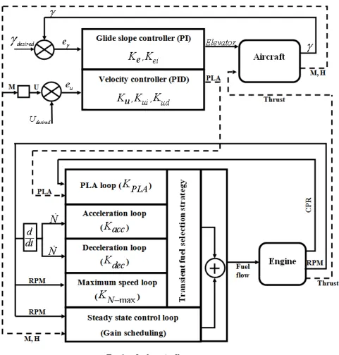
In this section, the engine fuel controller as we ll as the body glide slope and velocity controllers are described based on the engine control modes and flight simu lation control require ments. The structure of the controller is shown in Figure 5.

Figure 5. Engine and aircraft controllers’ structure

3.1. GTE Controller Design

The control of a gas turbine engine can be summarized by three different control modes including a steady state control mode to satisfy the pilot co mmand at steady-state condition, a transient control mode to regulate the time response of the engine, and a physical limitation control mode to fulfill the overspeed, over temperature and aerodynamic limitations.

In this paper, the fuel control system is designed based on an industrial strategy which divides the fuel flow into two parts including a steady state fuel flo w and a transient fuel flow[4, 24]. The engine steady state fuel flo w is defined for every equilibriu m point. The steady-state controller is respo

in Figure 5. The proportional gains of these control loops

named

K

_PLA

,

K

_dec

,

K

_acc

,

K

_Nmax respectively. 3.2. Airspee d and Flight Path Control

Airspeed is a critica l variable in the flight dynamics of an aircra ft. The a irspeed affects all o f the ae rodynamic forces and mo ments through the dynamic pressure. The airspeed controller uses a pitot tube to measure airspeed (u) and a PID controller to shape the control command which is sent to the throttle servo to adjust the propulsion power as follows:

( )

u

( )

( )

u u

u u i u d

e

s

PLA K e s

K

K

se s

s

=

+

+

(4)

Where

e s

_u

( )

=

U

_desired

( )

s

−

U s

( )

and Ku, Kui and Kud are the PID controller ga ins for the airspeed control system that must be tuned.

In addition the glide path, controller uses the pitch angle (θ) fro m the gyro and a PI controller to form the control command which is sent to the elevator servo. The glide path controller has the same structure as the altitude hold controller e xcept that the reference input is the glide path angle. So the Proportional-Integral controlle r of glide angle takes the following form

( )

( )

=

_e

+

_eie

s

Elevator

K e s

K

s

γ

γ (3)

Where

e s

_γ

( )

=

γ(s)-γ(s)

_desired and Ke and Kei are the PI

controller gains for the glide angle control system that must be tuned.

Both throttle and elevator affect the speed but the short and long-term effects of each of these controls are quite diffe rent. The throttle essentially affects the speed only in the short term but the elevator changes the steady-state speed. The schematic of the airc raft controlle rs is shown in Figure5. As it is observed in Figure5, there are 9 gains that must be tuned simultaneously for the engine and body control system.

3.3. Initial Gain Values

In order to select the initia l gain va lues for the 9 previously mentioned control loops, a manual tuning process is carried

out as follo ws: For GTE controller:

− The engine PLA loop gain (

K

_PLA) is firstly initia lized to achieve a preliminary response time . In order to improve

the engine response time,

K

_PLA is then increased until the process begins to oscillate. Then, in order to protect the

engine against surge, the

K

_{a cc} is changed until the

ma ximu m rotor speed derivative ( _N ) is limited to an allo wable va lue. After that, the

K

_decis changed until the minimu m rotor speed derivative ( _N ) is limited to an allo wable va lue. Consequently, the engine is protected against fla meout. Fina lly, in o rder to keep the engine integrity,

K

_N−maxis increased until the overspeed in every

condition are vanished without overshoot. For body controllers:

− The value of

K

_e is increased to achieve an acceptable

glide slope tracking. Ne xt, the

K

_{e i} value is increased to

eliminate the steady state error of glide slope tracking.

Subsequently, the values of

K K

u

,

u i

,

K

ud are changed in

the same ways until a reasonable velocity tracking is reached for the aircraft.

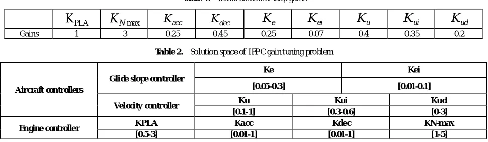
The initia l values obtained by the above process for a case study in Seal Level Standard (SLS) condition is shown in Table.1.

As mentioned earlier, the manual gain tuning process based on a trial and error manner may not result in an optimal controller fo r the airc raft and engine. Therefore, in order to achieve an imp roved performance for the engine and body simu ltaneously, the PSO method is proposed for IFPC gain tuning problem in this paper.

But, taking the iterative nature of PSO method into account, and since the IFPC controllers gain tuning proble m is a 9-d imensional optimizat ion proble m, the design variable ranges play in important role in computational effort of the optimization algorithm. Therefore , these ranges are restricted by a manual sensitivity analysis. Table (2) shows the lower and upper bound for the design variables.

Table 1. Initial controller loop gains PLA

K

K

_Nmax

K

acc

K

dec

K

e

K

ei

K

u

K

ui

K

ud

Gains 1 3 0.25 0.45 0.25 0.07 0.4 0.35 0.2

Table 2. Solution space of IFPC gain tuning problem

Aircraft controllers

Glide slope controller

Ke Kei

[0.05-0.3] [0.01-0.1]

Velocity controller Ku Kui Kud

[0.1-1] [0.3-0.6] [0-3] Engine controlle r KPLA Kacc Kde c KN-max

4. Problem Formulation

In this section, application of PSO fo r optimization of the previously described controllers is e xp lained. For this purpose, an overview of the method is firstly presented. The controller gain tuning procedure is then formu lated as an optimization proble m. Finally the PSO method is applied and the results are analyzed in the ne xt section. The effect of neighbor acceleration factor on PSO results is also investigated in this paper.

4.1. Par ticle Swar m Opti miz ation (PSO)

Partic le swarm optimization is a method for performing numerical optimization without explicit knowledge of the gradient of the problem to be optimized. PSO is attributed to Kennedy, Eberhart and Sh i[9] who are the founders of the fie ld. Origina lly intended for simu lating social behavior, the algorith m has been simplified after the partic les have been observed to be performing optimizat ion. The book by Kenne dy and Eberhart describes many philosophical aspects of PSO and swarm intelligence[5].

PSO shares many similarities with evo lutionary computat ion techniques such as GA. The system is init ia lized with a population of random solutions and searches for optima by updating generations. However, unlike GA , PSO has no evolution operators such as crossover and mutation. In PSO, the potential solutions, called particles, fly through the problem space by following the current optimu m partic les. More details can be found in[6, 25, 26].

One of the main advantages of PSO is that the PSO has few para meters to adjust and therefore is easy to imp le ment. PSO has been successfully applied in many areas including function optimization, art ificia l neura l network tra ining, fuz zy system control, and other areas where GA can be applied. This study suggests the PSO for IFPC optimization for the first time.

In this method, each part icle re fers to a point in a mu lti dimensional space whose dimension is related to the number of design parameters. The positions of points are changed in moves (iterations) with velocit ies which are calculated in

each step. In the first step, position

x

i_oand velocity

v

i_o for each point are generated randomly by upper and lower bounds of variable using the following equations:

min

(

max min

)

i o

x

=

x

+

rand x

−

x

(6)

max min max min

(

) 2

(

)

i o

v

= −

x

−

x

+

rand x

−

x

(7) where

i o

x

position of th

i

particle in the first step, i

o

v

veloc ity of th

i

particle in the first step,

min

x

lowe r bound of variable,

max

x

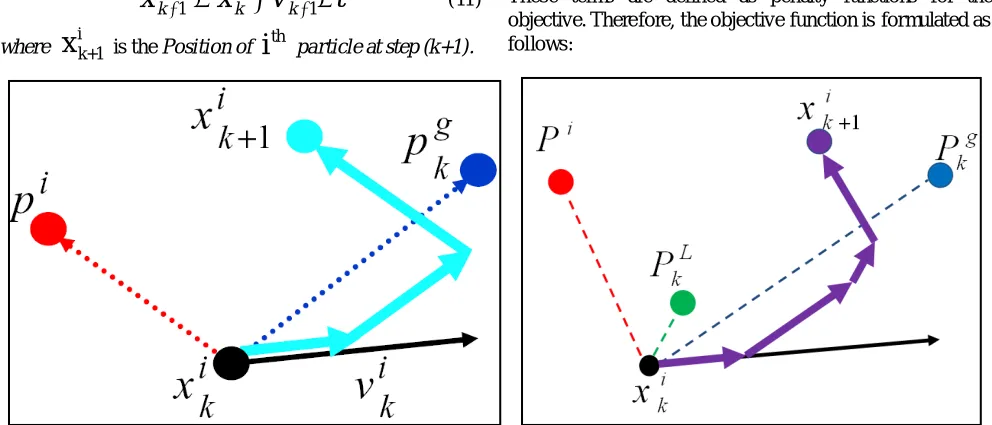
upper bound of variable ,

rand random variable between 0 & 1. As mentioned earlie r, the first population is distributed uniformly in the design space by this process. In the second step, PSO calcu lates new veloc ities to move the part icles fro m positions at time k to new positions at time k +1. For calculation of ne w velocit ies, three terms are needed:

• Inertia term: each partic le wants to continue its motion in its own current direct ion. Th is term is modeled by mu ltip lyi ng the particle’s current velocity vector by a number called inertia factor.

• Cognitive term: taking the self confidence characteristic into account, each particle has a velocity in the direction of its own best position over all the previous and current steps,

i

P

. This term is modeled by mult iplying the difference between the particle’s current position and the best position over all previous iterations by a number ca lled self confiden ce factor.

• _{Social term: each particle also gets effect fro m other}

particles. One part icle may be a ffected by the best position of

particles in the current swarm,

g k

P

_{, or by the best position}

of particles in its own vicinity,

P

k

L

. In the first case the algorith m is termed gBest PSO (global best) and in the second case it is termed LBest PSO (local best). The social confidence factor is used to model this term.

PSO e mp loys these three terms in addition to their corresponding coefficientsto calculate new velocities for the next iteration using a random distribution function. The coeffic ients inertia factor, self confidence factor and social confidence factor show the effect of the current motion, particle own me mory and swarm influence on the velocity vector of each particle, respectively.

The pseudo code of the procedure is as follows[11, 27]

For each particle Initialize particle End

Do

For each particle Calculate objective value

If the objective value is better than the best objective value (pBest) in history

set current value as the new pBest

End Choose the particle with the best objective value of all and/or some of particles as the gBest and/or lBbest

For each particle

Calculate particle velocity Update particle position End

Based on the above e xplanation, the velocity update formula takes the form (8) for g Best PSO and form (9) for LBest PSO:

1 1

(

)

2

(

)

i i i i g i

k k k k k

v

₊

=

wv

+

c rand P

−

x

+

c rand P

−

x

(8)

1 1

(

)

3

(

)

i i i i L i

k k k k k

where:

w

_{Inert ia factor,}

i k

v

Veloc ity of

i

thpartic le in the current motion,

1

c

Self confidence factor,

2

c

_{Socia l confidence factor (g Best),}

3

c

Social confidence factor (LBest),

i k

x

Position of

i

thparticle in current motion,

i

P

Best position of particle

i

thin current and all previous iterations,

g k

P

Position of the particle with best global objective at current iteration k,

L k

P

Best local neighbor position in the current iteration.

In this paper, the PSO approaches, take the effects of both gBest and Lbest in the velocity equation. In this case, the approach is referred to as neighbor acceleration effect. This modification is imp le mented in order to improve the speed of convergence[20]. Consequently, the velocity update formu la with neighbor accele ration effect ta kes the following form:

1 1 2

3

( ) ( )

( )

i i i i g i

k k k k k

L i k k

v wv c ra n d P x c ra n d P x c ra n d P x

+ = + − + −

+ −

(10)

Using the updated velocities vectors calculated by equation (4) and (5), the position of each particle is changed through the following equation:

1 1

i i i

k k k

x

₊

=

x

+

v

₊

∆

t

(11)

where

x

i_k+1 is the Position of

i

th particle at step (k +1).

This algorith m is repeated until a stopping criterion is reached. This criterion may be an ite ration number or a specified tolerance on the minimu m imp rovement of the best global value.

A schematic v iew of the position update of a part icle in gbest PSO and PSO with the neighbor acceleration effect is shown in Figure6. Moreover, in order to take both Lbest and gbest effect into account, a star social structure is defined for the swarm in this paper. Since a ll partic les are connected using this topology, each particle can be affected easily by a ll the particles or by its own neighbor. In this paper, neighbor hood is defined based on particles ind ices. In other words, neighbors of particle ith, are pa rtic les (i+1)th and particle (i-1)th . Another definition for neighborhood is presented by Suganthan, based on Euclidean distance[28].

4.2. Objecti ve Func tion

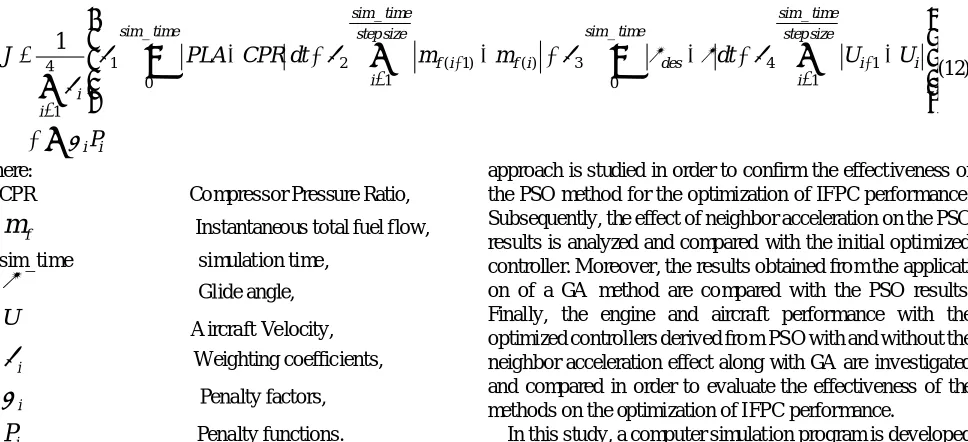
As mentioned earlier, the jet engine fuel controller, the aircra ft glide slope and velocity controlle rs are designed to satisfy GTE control modes including steady state, transient and physical limitation control modes as well as aircra ft control require ments. In other words, the objective o f the engine controller is to drive the GTE to the pilot desired set-point with good tracking with respect to flight path and speed require ments. Also, the objective of the body controller is to track the desired glide slope based on the specified a ircra ft maneuver as we ll as s mooth and reasonable variation of the speed with respect to safe operation of the engine. In both engine and body, the oscillation of parameters should be avoided. In addition, the engine must be protected from the physical limitations such as over speed, fla me out, lean and rich blowout and surge in co mpressor. These terms are defined as penalty functions for the objective. There fore, the objective function is formulated as follows:

(a) (b)

_ _

_ _

1 2 ( 1) ( ) 3 4 1

4

1 1

0 0

1

1

sim time sim time

sim time step size sim time step size

f i f i des i i

i i

i i

i i

J

PLA CPR dt

m

m

dt

U

U

P

β

β

β

γ

γ

β

β

α

+ +

= =

=









=



−

+

−

+

−

+

−















+

∑

∑

∫

∫

∑

∑





(12)

where:

CPR Co mpressor Pressure Ratio,

f

m



Instantaneous total fuel flow, sim_time simulat ion time ,

γ

_{Glide angle,}

U

_{A ircra ft Ve locity,}

i

β

Weighting coeffic ients,

i

α

Pena lty factors,

i

P

Pena lty functions.

In equation (12), the performance indices are norma lized first and then weighted according to their importance by the coeffic ients of

β

_i.In this paper all of these coefficients are assumed the same (0.25). The first and second terms in the equation (12) are re lated to the engine para meters. The first term guarantees the PLA trac king. It is worth mentioning that what the pilot usually wants to achieve wh ile moving the thrust lever is to let the engine deliver a certain percentage of the thrust that is available at the current flight conditions[29]. Since thrust itself is not measurable in flight, the relative thrust command given by the PLA setting must be translated into a command change of a measured variable. The relative thrust corresponds very well to the CPR and this parameter can be used for thrust modulation in controller design. The second term in (12) is aimed at obtaining a smooth change in the fuel flo w, wh ich results in a s mooth variation of the engine operating para meters.

The third and fourth terms in (12) are related to the aircraft glide slope trac king and the smooth variat ion of a ircra ft

velocity respectively. The

α

_i are termed to penalty factors tuned manually to achieve the reasonable results and

i

P

are termed to physical limitation as mentioned earlier. Moreover, the design optimization variables are the

controllers loop gains inc luding

K

_Nmax,

K

_acc,

K

_dec, PLA

K

in engine controller,

K

_e

,

K

_{e i} in g lide slope

controller,

K

_u,

K

_{u i} and

K

_{u d} in velocity controller as shown in Figure5. In other words, these 9 variables are going to be tuned using PSO in order to minimize the objective function of equation (12).

5. Optimization Results and Analysis

In this section, the result obtained from the gain tuning

approach is studied in order to confirm the effect iveness of the PSO method for the optimization of IFPC performance. Subsequently, the effect of neighbor acceleration on the PSO results is analyzed and compared with the in itia l optimized controlle r. Moreover, the results obtained fro m the applicati on of a GA method are co mpared with the PSO results. Finally, the engine and aircra ft performance with the optimized controllers derived fro m PSO with and without the neighbor acceleration effect along with GA are investigated and compared in order to evaluate the effectiveness of the methods on the optimization of IFPC performance.

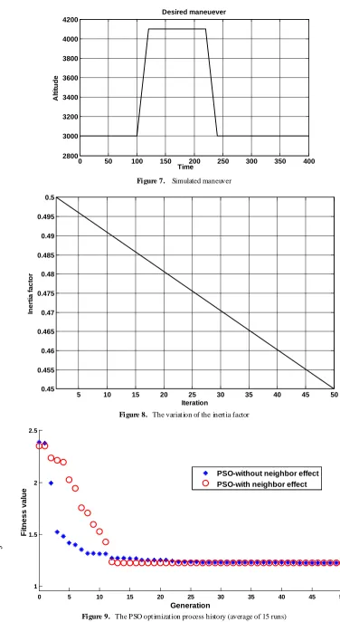
In this study, a computer simulat ion program is developed for a single spool turbojet engine integrated with a 6 D.O.F nonlinear flight simulat ion as a case study. Using each set of controller’s para meters, the time do ma in simulation is performed and the objective value is determined. The objective function is first evaluated by simulating the IFPC model considering a climb-cru ise-landing maneuver as shown in Figure 7.

5.1. PSO Results

In order to achieve an imp roved performance, the optimiz ation process has been run in a tria l and error manner with several PSO para meters to find the best set of parameters. The best results are achieved for the parameters presented in Table (3). It is worthwh ile to mention that there are some heuristic methods in the literature to find the PSO para meters. A study about these methods as well as their theoretical limitat ions can be found in[30, 31]. As shown in Table (3), the inertia factor decreases each iteration in order to transform the e xp loration nature o f the a lgorith m in the initia l runs to explo itation nature in the final runs. The variation of this factor is linear as shown in Figure8. The confidence factors are set to 1.5 and the neighbor factor is set to 0 fo r gbest PSO.

Moreover

, the we ight factors

0.25

i

β

=

, a re selected fo r the ob jective functions in equation (12). It means that the importance of the objectives is equal in the optimization p rocess. Optimizat ion is terminated in the prespecified nu mber of generations.

Table 3. Parameters used in PSO Swarm size = 100

Maximum Iteration = 50

c1 and c2 = 1.5 (confidence factors)

Wstart , Wend = 0.5, 0.45

Figure 7. Simulated maneuver

Figure 8. The variation of the inertia factor

Figure 9. The PSO optimization process history (average of 15 runs)

0 50 100 150 200 250 300 350 400

2800 3000 3200 3400 3600 3800 4000 4200

Time

A

lt

it

u

d

e

Desired maneuever

5 10 15 20 25 30 35 40 45 50

0.45 0.455 0.46 0.465 0.47 0.475 0.48 0.485 0.49 0.495 0.5

Iteration

In

er

ti

a f

act

o

r

0 5 10 15 20 25 30 35 40 45 50 1

1.5 2 2.5

Generation

F

it

n

ess val

u

e

PSO-without neighbor effect PSO-with neighbor effect

O

b

je

ctiv

e F

u

n

c

tio

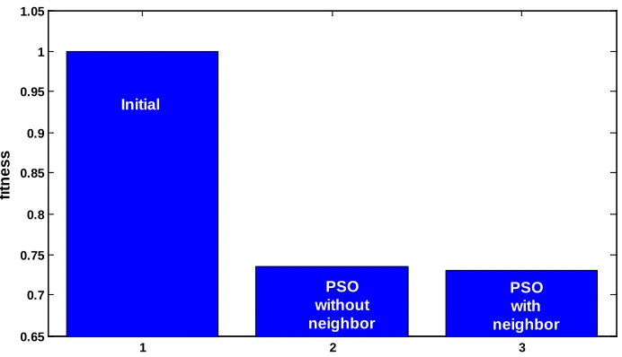
Figure 10. Objective function value for PSO (average of 15 runs)

In order to analyze the effect of the neighbor accelerat ion factor on the PSO results, the effect of the positions of the neighbor particles is a lso considered in this paper. For this purpose, the term with factor c3=1 isused in equation (10). Figure 9 shows the history of the objective function for both gbest PSO and PSO with neighbor effect. This Figure is derived fro m average of 15 runs of PSO with the Table (3) parameters. It is c lear fro m Figure 9 that, when the e ffect of neighbor acceleration is considered on the velocity update, the PSO converges faster (12 generations with neighbor acceleration effect against 28 generations without it). The faster convergence for the PSO with neighbor effect is due to more informat ion sharing a mong part icles. In other words, the particles degree of freedo m is increased using the neigh bor acceleration factor. It should be mentioned that increasing or decreasing of c 3 factor can increase or decrease the information sharing we ight between the particles respectively. The value of c3=1 causes the best results for the in hand problem. More details can be found in[18].

Genera lly , the lite rature reports that the gbest PSO conve rges faster than Lbest PSO because of better information sharing among the particles. The results of this paper show that the combined PSO (gbest PSO with neighbor effect) has better static convergence characteristics in comparison with gbest PSO for the problem at hand. Moreover, the neighbor effect gives a clustering character to the algorith m and prevents the solution from trapping in local optima.

Figure 10 shows the normalized objective function value respect to the value of initia l controller (controller with the gains presented in Table (1)). This Figure shows that the PSO method imp roves the objective value and confirms the effectiveness of the approach. The values of the objective function obtained from PSO with and without neighbor effect are appro ximately the same (about 26% imp rovement in co mparison with the initia l controller).

5.2. Comparison be twee n PSO and GA

In this section, the PSO results are compared with the

results obtained from the Genetic Algorith m (GA) in order to confirm the effectiveness of the proposed approach in optimization of IFPC gain tuning problem. The structure of simp le GA used in this paper is composed by an iterative procedure through the five ma in steps: To start the algorith m, an init ial population of individuals (ch ro mosomes) is defined. A fitness value is then associated with each individual, e xpressing the performance of the re lated solution with respect to a fixed object ive function (defined in equation (12)) to be min imized. Reproduction is then carried on as a p rocess of generating a ne w population fro m the current population. The ne xt step is selection, a mechanism for selecting the individuals with high fitness over low fitted ones to produce the new individuals for the next population. The variant used here is the roulette wheel method in wh ich the probability to choose a certain individual is proportional to its fitness. Subsequently, crossover and mutation are applied to the population as GA operators. Crossover is the method of me rging the genetic informat ion of two indiv iduals (parents) to produce the new individuals (ch ildren ). The scattered crossover method is used in this study. Mutation is a probabilistic random defo rmation of the genetic information for an individual. This process can be handled by altering each gene randomly with a s ma ll probability. The positive effect of mutation is the preservation of genetic diversity and that the local ma xima can be avoided. Following the evaluation of the fitness of all chro mosomes in the populatio n, the genetic operators are applied to produce a new population. After repetitions of the above operations, the new set of strings is obtained. This ends an iteration of the GA . Th is process is iterated and new populations are produced until a termination criterion is fulfilled. The GA was also run several times with various parameters for achieving the best results. Since the GA has more parameters than PSO, setting the best parameters for GA runs is mo re complicated than for PSO. Table (4) shows the best parameters of GA for the IFPC controllers gain tuning problem. In addition, the population size, initia l population

1 2 3

0.65 0.7 0.75 0.8 0.85 0.9 0.95 1 1.05

fi

tn

e

s

s

PSO with neighbor PSO

and stopping criterion are set to the same values in PSO and GA in order to co mpare the two approaches more prec isely. More details about the application of GA in aero-engine problem can be found in[32].

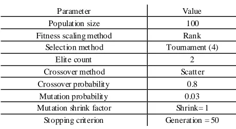
Table 4. Parameters used in GA

Parameter Value

Population size 100 Fitness scaling method Rank

Selection method Tournament (4)

Elite count 2

Crossover method Scatter Crossover probability 0.8

Mutation probability 0.03 Mutation shrink factor Shrink= 1

Stopping criterion Generation = 50

• Static convergence comparison

In order to investigate the ability of the proposed approach to find the global optima l solution, the dynamic programming (DP) method is also applied to the problem. The DP method works based on the princ iple of optima lity. It

should be mentioned that DP cannot give the controller parameters and only calculates the optimal control signal for the defined input PLA by breaking it down into simpler sub-problems in a recursive manner. The DP algorith m used in this paper is generated based on the theory presented by Dasgupta et al[33]. Table (5) co mpares the best objective value obtained from PSO and GA with DP. This table a lso shows the average of 15 runs. As it can be seen in this table, the objective value of the PSO is reasonably close to the objective value obtained from the global solution of DP. These results confirm that PSO provides almost the g lobal optima l value for this proble m. It seems that the GA method requires a para meters tuning process to achieve fitter results. Table (5) a lso co mpares the generation in wh ich the optimiz ation algorith ms find the fina l solution. As shown in this table, the PSO method converges faster than GA for the IFPC gain tuning proble m. It confirms the e ffectiveness of the proposed approach for IFPC controlle r design. However, it is worth mentioning that regarding the time consumption of all applied methods, the methodology used in this paper cannot imple mented in a rea l-t ime application.

Table 5. comparison between PSO and GA results (average of 15 runs) Method

(average of 15 runs) Initial GA

PSO (without neighbor)

PSO

(with neighbor) DP

Cost function value (Normalized) 1.5501 1.3573 1.2481 1.2476 1.2455

Optimization time (minute:second) - 52:25 38:20 38:45 254:00

Converge at generation number - 32 28 12 -

Figure 11. Standard deviation of population for PSO and GA

5 10 15 20 25 30 35 40 45 50

0 0.1 0.2 0.3 0.4 0.5 0.6 0.7 0.8 0.9 1

Generation (iteration)

S

tan

d

ar

d

D

evi

at

io

n

(

S

D

)

● Comparison of computational effort

As shown in table (5), the PSO run time is less than GA because of fewer fitness evaluations in PSO. Ta king the reduced number of para meters and the faster convergence of PSO into account, this table clearly demonstrates the simp li city of the PSO algorith m that resulted into huge saving in the computational efforts, in co mparison with other compara tively old and we ll-established techniques for population based evolutionary computations like the GA. In addition, another advantage of PSO is that PSO has fewer para meters to adjust and therefore is easy to imple ment.

● Dynamic convergence comparison

In order to co mpare the dynamic convergence of the used optimizat ion approaches, the standard deviation of populati on in each generation for the GA and PSO is plotted in Figure (11). These results are extracted fro m a typical run and it can be shown that this trend is similar for all runs. As shown in Figure 11, the dynamic convergence of PSO is considerably better than GA because GA uses mutation ope rator that increase the standard deviation.

The results presented in this section confirm the effective ness of PSO method in IFPC gain tuning as a rea l-world engineering optimization proble m. The co mparison between the PSO and GA results illustrates the relative merits of PSO fro m various points of view such as static and dynamic convergence and computational effort. Moreover, the PSO is easier to progra m in co mparison with GA . In addit ion, taking the effect of both gbest and Lbest into account, leads to improving the PSO results considerably. Therefore, the PSO method is reco mmended for the IFPC simultaneous gain tuning problem. The effect of the optimization process on IFPC performance is presented in the next section.

5.3. Effect of Opti miz ation on the IFPC Per for mance

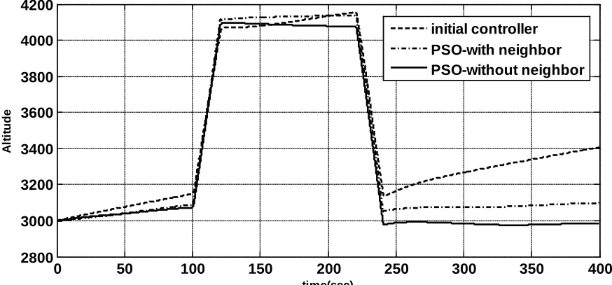
The PSO changes the IFPC loop gains and simu lates the engine and aircraft performance iterat ively until the stopping criteria o f the optimization prob le m are fulfilled. In order to verify and co mpare the effect iveness of the optimized contr olle rs, the perfo rmance o f the PSO with and without neighb or acceleration effect is tested for the specified maneuver. These results are compared with the results obtained from simu lation of the initia l controller with the gains presented in Table (1). As mentioned earlie r, a climb -cruise-landing man euver as shown in Figure 7 is e mployed in this study.

Figure 12 shows the variat ion of a ltitude during the mane uver. As shown in this Figure, the init ial controller cannot satisfy the maneuver altitude tracking. Both of PSO methods give good results in airc raft a ltitude control.

Figure13 shows the variation of aircraft speed. As shown in this Figure, the steady-state error is eliminated by the PSO methods. However, the PSO results with ne ighbor effect a re better than the PSO results without neighbor effect. The smooth variation of aircra ft speed around the desired magnit ude is also reached using the optimization method.

Figure 14 shows the glide angle trac king for the defined manuever using the initia l and the optimized controllers. As shown in this Figure, the results obtained from PSO show fast and acceptable response to the glide slope change, whereas the initial glide slope controller has a little lag to follow the specified g lide slope.

Figures 15 and 16 depict the engine performance. Figure 15 shows the PLA trac king of the GTE. Th is Figure shows that the results obtained from PSO outperform the init ial controller.

Figure 16 shows the engine rotor speed in climb – cruise - landing maneuver. Th is Figure shows the ability of the optimization approach to achieve an e fficient variation of RPM in this maneuver.

Figure 12. The variation of altitude through the maneuver

0 50 100 150 200 250 300 350 400

2800 3000 3200 3400 3600 3800 4000 4200

time(sec)

A

lti

tu

d

e

Figure 13. The variation of aircraft velocity through the maneuver

Figure 14. The glide angle tracking through the maneuver

Figure 15. The gas turbine engine PLA tracking through the maneuver

0 50 100 150 200 250 300 350 400

160 180 200 220 240

V

el

o

ci

ty

110 120 130 140 150 160 170 180 190 200 210

180 190 200 210

V

el

o

ci

ty

Desired Initial controller PSO-without neighbor PSO-with neighbor

0 50 100 150 200 250 300 350 400

-20 -10 0 10 20

G

li

d

e

s

lo

p

e

100 101 102 103

0 5 10 15

time(sec)

G

li

d

e

s

lo

p

e

220 221 222 223 224 225 -15

-10 -5 0

time(sec)

Desired initial controller PSO-without neighbor PSO-with neighbor

0 50 100 150 200 250 300 350 400

0.5 0.6 0.7 0.8 0.9

time(sec)

CP

R

98 100 102 104 106 108 110 112

0.65 0.7 0.75 0.8 0.85 0.9

time(sec)

CP

R PLA

Figure 16. The gas turbine engine rotor speed variation through the maneuver

Figure 17. The 3-D maneuver

Figure 18. The glide angle and velocity tracking through the 3-D maneuver

0 50 100 150 200 250 300 350 400

0.6 0.8 1

RP

M

102 104 106 108 110 112 114 116 118

0.85 0.9 0.95

time(sec)

RP

M

initial controller PSO-without neighbor PSO-with neighbor

0 0.5

1 1.5

2 2.5

3

x 104 0

5000 10000

15000 3000 4000 5000 6000 7000 8000

x (m) y (m)

z

(

m

)

0 50 100 150 200 250 300 350

-2 0 2 4 6

time (sec)

γ

(

de

g)

0 50 100 150 200 250 300 350

180 190 200 210 220

time (sec)

S

p

eed

(

m

/sec)

Desired tracking

Figure 19. The variation of gas turbine engine rotor speed and compressor pressure ratio through the 3-D maneuver

It can be observed fro m Figures.12-16 that both PSO without neighbor effect and PSO with neighbor effect outperform the init ial controlle r. The response with PSO is much faster, with less overshoot and settling time co mpared to the initia l controller. The responses of PSO with and without neighbor effect are a lmost similar, but the PSO with neighbor effect converges in fewer generations.

5.4. Reliability of Optimize d Controllers

Finally, to confirm the re liab ility of PSO method in optimization of IFPC proble m, the optimized controller is tested in a 3-dimensional challenging spiral maneuver as shown in Figure (17). This maneuver is carried on in 350 seconds. The optimized controlle r found by PSO with neighbor effect (in section 5.1) is used for this simulat ion.

Figure (18) shows the aircra ft para mete rs through the maneuver. As shown in this Figure, the optimized controller performs very we ll in trac king the glide slope as we ll as the desired velocity. This Figure proves the reliability of the optimized glide slope and velocity controller of the airc raft.

Also, Figure (19) shows the engine para meters through the maneuver. This Figure also shows the smooth variation of the engine CPR and RPM, which confirms the optimized operation of aero-engine as well as protection of the engine against physical limitations.

Figures 18 and 19 confirm the re liab ility of PSO as a swarm intelligence optimization method in simu ltaneous gain tuning of integrated flight and propulsion control as a challenging real-word optimization proble m. Finally, it should be mentioned that the tuned controller with fro zen gains performs well up to 7000 meter as shown in Figure17. Future studies can focus on other altitudes and also on noise rejection and load disturbance attenuation.

6. Conclusions

In this paper, application of PSO techniques is presented for the simultaneous IFPC gain tuning. PSO is applied to optimize a long term objective function in order to achieve a simu ltaneous acceptable performance for both engine and aircra ft. The results show that the PSO optimized controller

outperforms the initial controller in all object ive function terms. Moreover, co mparison between PSO and GA results confirms the e ffect iveness of PSO as an appropriate candida te to optimize the IFPC proble m in co mparison with other non-gradient based optimizat ion methods like conventional GA . In addition, the influence of the neighbor accele ration effect on the PSO performance is investigated in this paper. The results show that the neighbor acceleration factor has a considerable effect on the convergence rate of the PSO process. For this purpose, a computer simu lation is develope d for a single spool turbojet engine integrated with a 6 D.O.F nonlinear aircraft model to evaluate the objective function and to investigate the effectiveness of the approaches. For this optimizat ion proble m, the objective function is consider ed as a combination of the weighted PLA tracking and smooth response for the engine as well as glide slope tracki ng and velocity control for the airc raft. The results show that PSO can be used successfully for the optimizat ion of the IFPC para mete rs. The PSO has the advantage of fewe r para meters to adjust which ma kes it easy to imp le ment. Fina lly, the reliability of the optimized controller is illustrated using a 3-D spiral maneuver. In other words, the results of this paper show the successful application of PSO in an important aerospace control problem.

Abbreviations

Partic le swarm optimization (PSO)

Integrated flight and propulsion control (IFPC) Gas turbine engine (GTE)

Pilot lever angle (PLA)

Design Methods for Integrated Control Systems (DMICS) Dynamic progra mming (DP)

Genetic Algorithm (GA )

Proportional-Integral-Derivative (PID) Degree of Freedo m (D.O.F)

compressor pressure ratio (CPR)

REFERENCES

0 50 100 150 200 250 300 350

0 0.2 0.4 0.6 0.8 1

time (sec)

E

ngi

ne

C

P

R

0 50 100 150 200 250 300 350

0 0.2 0.4 0.6 0.8 1

time (sec)

E

ngi

ne

r

[1] Sanjay Garg and Duane L. M attern, R.E.B.: Integrated Flight /Propulsion Control System Design Bas ed on a Centralized Approach, N.T.M . AIAA-89-3520, (1989)

[2] Smith, K.L.: Design methods for integrated control systems. Wright Patterson AFB, OH, Rep. AFWAL-TR-86-210, (1986)

[3] Shaw, P.D., Rock, S.M ., and Fisk, W.S: Design M ethods for Integrated Control Systems, A.P.L. A F WAL-TR-88-2061 , Wright Patterson AFB, Dayton OH, Editor. (1988)

[4] A. Kreiner, K.L.: The use of onboard real-time models for jet engine control. M TU Aero Engines, Germany. p. 27. (2002) [5] Kennedy, J. And R. Eberhart.: Particle Swarm Optimization,

in Proceedings of the IEEE International Conference On Neural Networks, Perth, Australia(1995)

[6] Eberhart ,Yuhui Shi.: Particle Swarm Optimization, Develop ments, Applications and resources. IEEE, (2001)

[7] Eberhart ,Yuhui Shi.: A modified particle swarm optimizer, in IEEE Int. Conf. Evol. Comput., Anchorage, AK, pp. 69–73. (1998)

[8] Venter, G. and Sobieski, J.: Particle Swarm Optimization. AIAA 2002-1235, 43rd AIAA/ASM E/ASCE/ AHS/ASC Structures, Structural Dynamics, and M aterials Conference, Denver, CO., April (2002)

[9] Y. Shi and R. C. Eberhart.: Empirical study of particle swarm optimization, in Proc. IEEE Int. Conf. Evol. Comput., Washington, DC, pp. 1945–1950. July (1999)

[10] Zwe-Lee Gaing, M ., IEEE, A Particle Swarm Optimization Approach for Optimum Design of PID Controller in AVR System. IEEE transactions on energy conversion, vol. 19, no. 2, June (2004)

[11] Lin, C. O. W.: Comparison between PSO and GA for Parameters Optimization of PID Controller, in Proceedings of the IEEE International Conference on M echatronics and Automation June 25 - 28, Luoyang, China. (2006)

[12] M ajid Zamani, Nasser Sadati, and M asoud Karimi Ghartema ni.: Design of an H∞ PID Controller Using Particle Swarm Optimization. International Journal of Control, Automation, and Systems (2009)

[13] M . R. Yousefi, S.A.E., S. Eshtehardiha, and M . Bayati Poudeh,: Particle Swarm Optimization and Genetic Algorithm to Optimizing the Pole Placement Controller on Cuk Converter, in 2nd IEEE International Conference on Power and Energy (PECon 08), December 1-3, Johor Baharu, M alaysia. (2008)

[14] H´ajek , Parameterization of Airfoils and Its Application in Aerodynamic Optimization, WDS'07 Proceedings of Contributed Papers, Part I, 233–240, (2007)

[15] C. Praveen, R. Duvigneau,: Low cost PSO using metamodels and inexact pre-evaluation: Application to aerodynamic shape design, Comput. M ethods Appl. M ech. Engrg. 198 (2009) [16] Bessette, CR, and Spencer, DB: Isentifying Optimal interpla

netary trajectories Through a Genetic Approach, AIAA 2006-6306 AIAA/AAs Astrodynamics (2006)

[17] Bessette, CR, and Spencer, DB: Optimal space trajectory Design: A Heuristic-Based Approach, Advances in Astronau

tical Sciences, Univelt inc., San Diego, CA, 124, 1611-1628; AAS paper 06-197 (2006)

[18] M orteza Montazeri-Gh, Soheil Jafari, M ohammad R.Ilkhani.: Application of Particle Swarm Optimization in Gas Turbine Engine Fuel Controller Gain Tuning, Engineering Optimizati on, http://dx.doi.org/10.1080/0305215X.2011.576760. Vol. 44, No. 2, February 2012, 225–240 (2012)

[19] Tony Giampaolo, M., PE,: Gas Turbine Handbook: Principles and Practices. Fairmont Press, Inc. (2006)

[20] A.Thompson, G.G.K.a.H.: Dynamic M odeling of Gas Turbines. Industrial control center, Glasgow, scotland, U.K. (2003)

[21] M ontazeri-Gh. M , Safarabadi-f.M ,: M odeling and simulation of gas turbine engine performance in order to design of fuel control system design (in Persian). International Journal of Engineering Science (IJES) vol.19, No.10. (2008)

[22] Evans, C.: Testing and modeling aircraft gas turbines: an intr oduction and overview, in UKACC International Conference on Control. Conference Publication No. 455. (1998)

[23] M . M ontazeri-Gh, S.M ojallal.: M odeling and simulation of gas engine performance, in M ESM Sharjah. (2002)

[24] H. Austin Spang, H.B.: Control of jet engines. Control Engineering Practice, p. 17. (1999)

[25] Fei Gao, H.T.: Particle Swarm Optimization: An efficient M ethod for Tracing Periodic Orbits and Controlling Chaos, in Proceedings of the International Conference on Complex Systems and Applications. Watam Press. (2006)

[26] Engelbrecht, A.: Particle Swarm Optimization Pitfalls and convergence Aspects, in Department of computer science, University of Pretoria, South Africa. (2005)

[27] Sidhartha Panda, N.P.P.: Comparison of Particle Swarm Optimization and Genetic Algorithm for TCSC-based Controller Design. International Journal of Computer Science and Engineering, (2007)

[28] Suganthan, P. N.: Particle Swarm Optimizer with Neighborh ood Operator. In Proceeding of the IEEE congress on Evolutionary Computation, Paged 1958-1962. IEEE press (1999)

[29] Cohen, H., Rogers, G. F. C., & Saravanamuttoo, H. I. H., Gas turbine theory, ed. t. ed. Essex: Longman. (1996)

[30] Perez, R.E. and Behdinan, K.: Particle swarm approach for structural design optimization", Computers and Structures, Vol. 85, pp. 1579-1588 (2007)

[31] Sedighizadeh, D., M asehian, E.: Particle swarm optimization methods, taxonomy and

applications", International Journal of Computer Theory and Engineering, Vol. 1, pp. 1793-8201, (2009)

[32] M . M ontazeri-Gh and S. Jafari,: Evolutionary Optimization for Gain Tuning of Jet Engine M in- M ax Fuel Controller, JOURNAL OF PROPULSION AND POWER, Vol. 27, No. 5, September–October (2011)