Volume 12, Number 2, pp. 275–282. http://www.scpe.org c 2011 SCPE
SOME GEOMETRIC PROBLEMS ON OMTSE OPTOELECTRONIC COMPUTER
SATISH CH. PANIGRAHI∗AND ASISH MUKHOPADHYAY†
Abstract. Optical Multi-Trees with Shuffle Exchange (OMTSE) architecture is an efficient model of an optoelectronic com-puter. The network has a total of 3n3/2 nodes. The diameter and bisection width of the network are 6 logn−1 and n3/4
respectively. In this note, we present synchronous SIMD algorithms on an OMTSE optoelectronic computer for the following prob-lems in computational geometry: Convex Hull, Smallest Enclosing Rectangle, All-Farthest/All-Nearest Neighbors, Closest/Farthest pair, Maximal Points. The strength of the proposed algorithms over the existing algorithms on OMULT has also been discussed.
Key words: Parallel Algorithms, Optoelectronic Computer, Computational Geometry, OTIS Mesh, OMULT
1. Introduction. Optical interconnections are superior in power, speed with less crosstalk properties as compared to electronic interconnections when the interconnection distance is more than a few millimeters [1, 6]. Motivated by these observations, some new hybrid optoelectronic computer architectures utilizing both optical and electronic technologies have been proposed and investigated by several researchers [8, 10, 13, 15]. In these architectures, both the electronic link and the optical link are done where the former is being considered within the same physical package (e.g. chip) where as the latter is for the pair of processors that are kept in different packages.
A number of parallel algorithms on these optoelectronic computers have been addressed and studied exten-sively [3, 4, 5, 7, 8, 9, 10, 14]. In this paper we present some computational geometry algorithms such as Convex Hull, Smallest Enclosing Rectangle, All-Farthest/All-Nearest Neighbor, Closest/Farthest pair, Maximal Points, on OMTSE optoelectronic computer [8, 10]. Irrespective of different factor network of OMTSE than OMULT, here in this paper we show that Convex hull and Smallest Enclosing Rectangle problem for n points can be solved on OMTSE inO(logn) time with the same time complexity as on OMULT [2]. Here it is worth noting that the total number of processors of OMULT and OMTSE respectively beδ1 =n2(2n−1) andδ2 =n2(3n
2 )
(we haveδ1< δ2, as because of their topological nature we can assume that n≥4). Islam et al. in [2] stated that algorithm for empirical cumulative distribution, all nearest neighbor can be implemented on OMULT in
O(logn) time for n number of points. In this paper we explore this line of work farther and implement the algorithms such as All-Farthest/All-Nearest Neighbor, Closest/Farthest pair amongn2points inO(nlogn) time
and also provide an algorithm for maximal points amongn3data points in O(logn) time.
The rest of the paper is organized as follows. In section 2 we briefly present the topological property of the OMTSE System. In section 3, we describe our propose algorithms and finally we conclude in section 4.
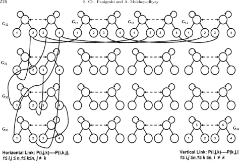
2. Topology of OMTSE. The factor network used in OMTSE topology constitutes two layer Trees with Shuffle Exchange (TSE) network. The TSE is nothing but an interconnection network containing a group of 2k, k ≥1, complete binary trees of height one and the roots of these binary trees are connected with Shuffle-Exchange fashion. The OMTSE interconnection system consists of n2 TSE networks, which are organized in
the form of ann×ngrid in matrix form. We denote the TSE network placed atithrow andjthcolumn of this matrix byGij,1≤i, j≤n. Each TSE network hasnnodes at layer 2 andn/2 nodes at layer 1 which results in N = 3n3/2 processors in total. The nodes within each TSE network are interconnected by usual electronic links,
while the nodes at layer 2 (i.e. the layer having leaf processors) of different TSE networks are interconnected by optical links according to the rules defined below. Let us label the nodes in each TSE networkGij,1≤i, j≤n, by distinct integers from 1 to 3n/2 in reverse order, i.e., the nodes at both layer 2 and 1 of TSE network are numbered from 1 to 3n/2 in order from left to right. The node,k, in a TSE networkGij will be referred as the processorP(i, j, k),1≤i, j ≤n,1≤k ≤3n/2. We can now define the optical links interconnecting only leaf nodes in different TSE networks in the following way.
∗School of Computer Science, University of Windsor, Canada([email protected]). †School of Computer Science, University of Windsor, Canada([email protected])
Fig. 2.1: An example of OMTSE topology with n = 4
(1) ProcessorP(i, j, k),1≤i, j, k≤n, j6=k,is connected to the processorP(i, k, j) by bi-directional optical link called horizontal inter-TSE link.
(2) ProcessorP(i, j, k),1≤i, j≤n, i6=k, is connected to the processorP(k, j, i) by bi-directional optical link called vertical inter-TSE link.
The diameter of a network is defined as the maximum distance between any two processing nodes in the network. If we start from a node P(i, j, k),1 ≤ i, j ≤ n,1 ≤ k ≤ 3n/2, we can reach another node
P(i′, j′, k′),1≤i′, j′≤n,1≤k′≤3n/2,of the OMTSE interconnection system by traversing the path
P(i, j, k)→P(i, j, j′)→P(i, j′, j)→P(i, j′, i′)→P(i′, j′, i)→P(i′, j′, k′)
It can easily be seen that the diameter of OMTSE topology is 6 logn−1 which is O(logn) comprising of 6 logn−3 electronic links and 2 optical links. Similarly we can find out the bisection width of OMTSE topology is equal ton3/4. An Example of OMTSE topology forn= 4 with partial links is shown in FIG. 2.1.
3. Proposed Algorithms.
3.1. Convex Hull. The convex hull [11] of a set of points S in the plane is smallest convex polygonP
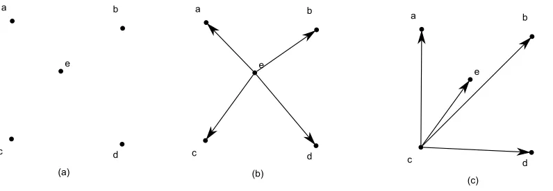
that encloses S, smallest in the sense that there is no other polygonP′ such that P ⊃ P′ ⊇ S. To find the convex hull for a given set of points S on a plane we need to identify the extreme points, in particular, what constitutes constructing the boundary. Suppose|S|=nand assume that no three points in S are collinear then our algorithm employs the result of the following theorem discussed in [14].
a b
c d
e
(a)
a b
c d
e
(b)
a b
c d
e
(c)
Fig. 3.1: Example for Theorem 3.1:(a) Original Layout, (b) pi=e, (c)pi=c
We assume that each leaf processor P(i, j, k)(1 ≤ i, j, k ≤ n) has three registers, represent by A(i, j, k),
B(i, j, k) and C(i, j, k). We have a set of pointsS =p1, p2, ..., pn in which no three points are collinear. The coordinates of all n points are initially stored in the A-register of the leaf nodesG11.
Algorithm: ConvexHull()
Input: ∀k,1≤k≤n A(1,1, k)←pk Output: ∀k,1≤k≤n
Extreme points ←B(1, 1, k)
Step 1: ∀i, j; 1≤i, j≤n,do in parallel
Broadcast all these n points to the A-register of the respective leaf nodes ofGij [9].
Step 2: ∀i, j, k; 1≤i, j, k≤n,do in parallel
Broadcast the point in the A-register ofP(i, j, i) to all theB(i, j, k) ofGij.
Step 3: ∀i, j, k; 1≤i, j, k≤n,do in parallel
Compute the polar angle of the vectorpi→pik atP(i, j, k) ofGij and store inC(i, j, k) along with the zero vector.
Step 4: ∀i, j, k; 1≤i, j, k≤n,do in parallel
Sort thenvectorspi→pik stored in the C-register of the leaf nodes of each Gij. After this step we assume the sorted order list given by eachGij is pipi1, pipi2, ..., pipin(i.e. in eachGij the vector
→
pipi1 always represent the
zero vector.)
Step 5: ∀i, j, k; 1≤i, k≤n,and 2≤j≤n,do in parallel Broadcast the content ofC(i, j, j) toA(i, j, k). Step 6: ∀i; 1≤i≤n,do in parallel
i)∀j,2≤j≤n−1,
Calculate the counter clockwise angle betweenpi→pij and
→
pipi(j+1) at each Gij and store the result inC(i, j, j+ 1)
ii)∀j, j=n,
Calculate the counter clockwise angle betweenpi→pin and
→
pipi2 at eachGin and store it inC(i, n,2).
Step 7: ∀i; 1≤i≤n, do in parallel i)∀j;j = 1
ii)∀j; 2≤j≤n−1 if ((C(i, j, j+ 1)> π))
C(i, j,1)←1. else
C(i, j,1)←0. iii)∀j;j=n
if ((C(i, n,2)> π))
C(i, n,1)←1. else
C(i, n,1)←0.
Step 8: ∀i, j; 1≤i, j≤n, do in parallel
C(i,1, j)←C(i, j,1). /∗through the horizontal optical link content of
C(i, j,1) is moved toC(i, j,1)∗/
Step 9: ∀i, k; 1≤i, k≤n, do in parallel if (C(i,1, k) == 0)
B(i,1,1)←N U LL. /∗ if the content of C-register of all leaf nodes ofGi1
is 0 then resetB(i,1,1) to NULL value∗/
Step 10: ∀i,1≤i≤n,do in parallel
B(1,1, i)←B(i,1,1). /∗through the vertical optical link content of
B(i,1,1) is moved to B(1,1, i)∗/
Hence the extreme points of the convex hull can be taken from the B-register of all leaf nodes of G11
excluding the NULL entries. In order to analyze the time complexity of the above algorithm we also consider the data movements along the both electronic link and optical link. For the complete group broadcast [9] the step 1 needs 4 logn−2 electronic moves and 3 optical moves. For the required intra-group group broadcast [8] the step 2 and 5 need 2 logn−1 electronic move. For the basic assignment and geometry operations we can assume that the steps 3, 6, 7 and 9 need O(1) time. The required sorting (see appendix) ofnpoints at corresponding
Gij,1≤i, j ≤nthe step 4 needs 7 logn−1 electronic move and 5 optical move. In addition, for the required inter-group data movement the step 8 and 10 need one optical move. Thus overall, we needO(logn) to compute the convex hull.
Theorem 3.2. Algorithm PCH requires O(logn)time to compute the convex hull of npoints.
The above algorithm can be extended for the smallest enclosing rectangle ofnpoints withinO(logn) time as discussed in [2]. But it would be interesting to devise algorithm for convex hull and smallest enclosing rectangle amongn2 data points on both OMULT and OMTSE optoelectronic computer.
3.2. All-Nearest/All-Farthest Neighbor. All-Nearest(All-Farthest) Neighbor problem can be stated as follows: given a set S = {p1, p2, ..., pq} of q points, for each point pi ∈ S we wish to determine a point pj∈ {S−pi} such that the Euclidean distancekpi−pjkis minimum(maximum).
In order to implement All-Nearest Neighbor (All-Farthest Neighbor can be dealt analogously) problem for
n2 points, we assume that each leaf processorP(i, j, k),1≤i, j, k≤n, has four registers A, B, C and D; where
as each non-leaf processorP(i, j, k),1≤i, j≤n, n+ 1≤k≤3n
2, has two registers A and B. Initially, the points p(i−1)+k is stored in the A(i, i, k)of all the diagonal leaf nodes of Gii,1≤i ≤n, where as all the D-registers of OMTSE system are set to zero. Set a counter variablec to zero at B-register of each non leaf processor of OMTSE optoelectronic system. Here we describe the algorithm in the following steps
AlgorithmAllN earestN eighbor() Input: ∀i, k,1≤i, k≤n
A(i, i, k)←p(i−1)+k Output: ∀i, k,1≤i, k≤n
Nearest Neighbor ofp(i−1)+k ←C(i, i, k)
Step 2.1: ∀i, j,1≤i, j≤n, do in parallel if (c== 0)
Broadcast the content ofA(i, j, i) to B-registers of all leaf nodes ofGij. else
Broadcast the content ofB(i, j,1 + (j%n)) to B-register of all leaf nodes ofGij.
Step 2.2: ∀i, j, k,1≤i, j, k≤n, do in parallel
D(i, j, k)← kA(i, j, k)−B(i, j, k)k
if (D(i, j, k) == 0)
D(i, j, k)← ∞
Step 2.3: ∀i, j, k,1≤i, j, k≤n, do in parallel
Compute the minimum of values stored in each D-register ofGij and store the result inC(i, j,1 + ((j+c−1)%n)).
Step 2.4: ∀i, j, k,1≤i, j, k≤n,do in parallel
Perform horizontal optical move on the content of B-registers so that the data from each side move to the corresponding leaf nodes. Step 2.5: ∀i, j, k,1≤i, j≤n, n+ 1≤k≤ 3n
2, do in parallel c=c+ 1.
Step 3: ∀i, j, k,1≤i, j, k≤nand j6=k, do in parallel
Perform horizontal optical move on the content of C-registers so that the data from each side move to the corresponding leaf nodes.
Step 4: ∀i, k,1≤i, k≤n, do in parallel
Compute the minimum of values stored in each C-register ofGki and store the result inC(k, i, i).
Step 5: ∀i, k,1≤i, k≤nandi6=k, do in parallel
C(i, i, k)←C(k, i, i)/∗Vertical Optical Move∗/
For the required column group broadcast the step 1 requires 2 logn−1 electronic moves and 3 optical moves. The Step 2.1 requires 2 logn−1 electronic moves for intergroup broadcast. To find the minimum in each groupGij, the step 2.3 and step 4 requireO(logn) time. Again the Step 2.4, Step 3 and Step 5 require one optical move each. For the basic increment and distance measure we can assume that the Step 2.2 and Step 2.5 requireO(1) time. Since we have n iterations of while loop in Step 2, the overall complexity of the algorithm is
O(nlogn) forn2 points.
3.3. Closest-Pair/Farthest-Pair of Points. This problem can be defined as follows: given a set S =
{p1, p2, ..., pq} of q points, ∃{pi, pj} ∈S such that euclidean distance kpi−pjk is minimum(maximum). The closest pair of points can be found by first solving the All-Nearest neighbor problem and then determining the closest pair among the nearest problem of each point. Here we describe the basic algorithm for n2 points in
following steps
Algorithm: ClosestP airP oints()
Input: ∀i, k,1≤i, k≤n A(i, i, k)←p(i−1)+k Output: Closest-pair←C(1,1,1)
Step 1: AllN earestN eighbor() Step 2: ∀i,1≤i≤n
Compute the minimum at eachGii and store the result inC(i, i,1) Step 3: ∀i,1≤i≤n
C(1, i, i)←C(i, i,1) Step 4: ∀i,1≤i≤n
C(1, i,1)←C(1, i, i)
The algorithmClosestP airP ointsrequire additional 3 logn−1 electronic moves and 2 optical moves which will be subsumed by theO(nlogn) ofAllN earestN eighboralgorithm.
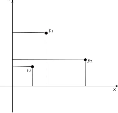
3.4. ECDF. In ECDF (empirical cumulative distribution function) problem [14], we are given a set S=
{p1, p2, ..., pq} of q distinct points. For{pi(xi, yi), pj(xj, yj)} ∈S, we will say pi dominatespj iffxi ≥xj and yi ≥yj. For allpi ∈ S, we are going to determine the number points it dominates in set S. In the FIG 3.2 we have illustrated a dominating relationship between three points p1,p2, andp3. In this case, the number of points dominated byp1, p2 andp3, respectively are 1, 1, and 0.
X Y
Fig. 3.2: Example of dominating relation
The algorithm to implement ECDF forn2 is quite similar to theAllN earestN eighboralgorithm. Here in
order to get dominating value of pointp(i−1)+k at correspondingC(i, i, k), in step 2.2 ofAllN earestN eighbor algorithm the D-register value is set to 1 if B-register point dominates its A-register point. Then in Step 2.3, we need to compute the summation of all D-register value with in that group and store the result in
C(i, j,1 + ((j+c−1)%n)). After this the D-register is reset to zero and contiue the loop whilec < n. Further, in Step 4 we need to compute the summation of values stored in each C-register ofGki and store the result in C(k, i, i). Finally in Step 5 we get the dominating value of pointp(i−1)+k at corresspondingC(i, i, k).
To compute the summation in shuffle exchange network [12] takes the same complexity as to compute the minimum. Thus the time taken to implement ECDF for n2 points is same as that of AllN earestN eighbor
algorithm i. e. O(nlogn).
3.5. Two-Set Dominance. The two set dominance problem can stated in this way: We have given two sets S1={p1, p2, ..., pp}and S2 ={q1, q2, ..., qq}, for each pointpi ∈S1(or qj ∈S2) we wish to determine the number points inS2(or S1) is dominated bypi(or qj). This is quite similar to the ECDF and can be achieved withO(nlogn) forkS1+S2k=n2 points.
3.6. Maximal Points. A pointp∈S is maximal iff it dominates all the points in S. This is quite simple and can be achieved byO(logn) time forkSk=n3points as follows.
Algorithm: M aximalP oint
Input: Arbitrarily assign then3 points ton3 leaf processors of OMTSE
optoelectronic computer. Output: Maximal point←A(1,1,1) Step 1: ∀i, j,1≤i, j≤n,
Each groupGij determine the maximal point with in that group and store the result inA(i, j,1)
A(i,1, j)←A(i, j,1) Step 3: ∀i,1≤i≤n,
Each groupGi1 determine the maximal point with in that group and store
the result inA(i,1,1) Step 4: ∀i,1≤i≤n,
A(1,1, i)←A(i,1,1)
Step 5: The groupG11 determine the maximal point with in that group and store the result inA(1,1,1)
For finding the local maximal points with in a group, the Step 1, 3 and 4 requiresO(logn) electronic moves each. Further, for the inter group communication we require one optical move each for the Step 2 and 4. Thus overall we haveO(logn) algorithm with exactly 3 lognelectronic moves and 2 optical moves. Now if we define minimal points analogous to maximal points, the above algorithm can be improved slightly to get both the maximal and minimal points out ofn(n−1)2 points with 4 logn+ 4 electronic moves and 3 optical moves as
discussed in [10].
4. Conclusion. We have shown that several computational geometry problems can be solved on OMTSE optoelectronic computer efficiently. It would be interesting to devise the discussed algorithms forn3number of
points on OMTSE and OMULT system.
Acknowledgments. This research is supported by an NSERC Individual Discovery Grant to second au-thor.
REFERENCES
[1] M. R. Feldman, S. C. Esener, C. C. Guest, and S. H. Lee,Comparison between optical and electrical interconnects based on power and speed considerations, Appl. Opt., 27 (1988), pp. 1742–1751.
[2] R. Islam, N. Afroz, S. Bandyopadhyay, and B. P. Sinha, Computational geometry on optical multi-trees (OMULT) computer system, in CCCG, 2005, pp. 150–154.
[3] P. K. Jana,Improved parallel prefix computation on optical multi-trees, in India Annual Conference, 2004. Proceedings of the IEEE INDICON 2004. First, 20-22 2004, pp. 414 – 418.
[4] P. K. Jana,Polynomial interpolation and polynomial root finding on otis-mesh, Parallel Computing, 32 (2006), pp. 301–312. [5] P. K. Jana and K. Sinha,Permutation algorithms on optical multi-trees, Comput. Math. Appl., 56 (2008), pp. 2656–2665. [6] A. V. Krishnamoorthy, P. J. Marchand, F. E. Kiamilev, and S. C. Esener,Grain-size considerations for optoelectronic
multistage interconnection networks, Appl. Opt., 31 (1992), pp. 5480–5507.
[7] D. K. Mallick and P. K. Jana,Parallel prefix on mesh of trees and otis mesh of trees, in PDPTA, H. R. Arabnia and Y. Mun, eds., CSREA Press, 2008, pp. 359–.
[8] S. C. Panigrahi, S. Paul, and G. Sahoo,OMTSE - an optical interconnection system for parallel computing, in Advanced Computing and Communications, 2006. ADCOM 2006. International Conference on, 20-23 Dec 2006, pp. 626 –627. [9] ,Parallel prefix computation, sorting and reduction operation on OMTSE architecture, in ICACC 2007 International
Conference, 9-10 Feb 2007, pp. 616 –622.
[10] S. C. Panigrahi and G. Sahoo,An MIMD algorithm for finding maximum and minimum on OMTSE architecture, Scalable Computing: Practice and Experience, 9 (2008), pp. 69–75.
[11] F. P. Preparata and M. I. Shamos,Computational geometry: an introduction, Springer-Verlag, New York, 1985. [12] M. J. Quinn,Parallel computing (2nd ed.): theory and practice, McGraw-Hill, Inc., New York, NY, USA, 1994.
[13] B. P. Sinha and S. Bandyopadhyay, OMULT: An optical interconnection system for parallel computing, in Euro-Par, M. Danelutto, M. Vanneschi, and D. Laforenza, eds., vol. 3149 of Lecture Notes in Computer Science, Springer, 2004, pp. 856–863.
[14] C.-F. Wang and S. Sahni,Computational geometry on the OTIS-mesh optoelectronic computer, in ICPP, IEEE Computer Society, 2002, pp. 501–.
[15] F. Zane, P. Marchand, R. Paturi, and S. Esener,Scalable network architectures using the optical transpose interconnection system (OTIS), J. Parallel Distrib. Comput., 60 (2000), pp. 521–538.
Appendix
AlgorithmSort()
Step 1: Perform a column broadcast [8] so that the list of elements stored in the leaf nodes ofG11broad casted to the corresponding leaf nodes allGi1,1≤n. Step 2: ∀i,1≤i≤n, do in parallel
Broadcast the elementaito R2-register of all leaf nodes ofGi1. Set a Flag as 1 ifaigreater than other element in R1-register of same leaf node. Otherwise set Flag as zero. The value of the Flag variable can be kept in R2-register which may overwrite previous entries.
Step 3: ∀i,1≤i≤n, do in parallel
Compute the summation of all Flag values stored on each leaf nodes ofGi1, which is the rank(r) of the elementai in the given list.
Remark: As a result of summation in the shuffle exchange network [12] the rank value will reflect in all nodes of shuffle exchange layer ofGi1.
Step 4: ∀i,1≤n, do in parallel
if the rank of aiis r then the elementaiis moved toR1(i,1, r). Step 5: ∀i,1≤n, do in parallel
R1(r,1, i)←R1(i,1, r)/∗Vertical optical link∗/
Step 6: ∀i,1≤n, do in parallel
R1(r,1,1)←R1(r,1, i) Step 7: ∀r,1≤r≤n, do in parallel
R1(1,1, r)←R1(1,1, r)/∗Vertical optical link∗/
For the complexity analysis of the above algorithm we also consider the data movement along the electronic and optical link. The above algorithm needs (7 logn−1) communication steps along electronic links and 5 communication steps along optical links [8] giving overallO(logn) time algorithm. The idea can be extended to sortn2
data values in
O(nlogn) time but this is beyond the scope of this paper.
Edited by: Dana Petcu and Marcin Paprzycki
Received: May 1, 2011