Methods for Constructing a Yield Curve

Methods for Constructing a Yield Curve

input is perturbed (the method is not local). In Hagan and West [2006] we introduced two new interpolation methods—the monotone convex method and the minimal method. In this paper we will review the monotone convex method and highlight why this method has a very high pedigree in terms of the construction quality crite-ria that one should be interested in.

Keywords

yield curve, interpolation, fixed income, discount factors

Abstract

In this paper we survey a wide selection of the interpolation algorithms that are in use in financial markets for construction of curves such as forward curves, basis curves, and most importantly, yield curves. In the case of yield curves we also review the issue of bootstrapping and discuss how the interpolation algorithm should be in-timately connected to the bootstrap itself.

As we will see, many methods commonly in use suffer from problems: they posit un-reasonable expections, or are not even necessarily arbitrage free. Moreover, many methods result in material variation in large sections of the curve when only one

1 Basic Yield Curve Mathematics

Much of what is said here is a reprise of the excellent introduction in [Rebonato, 1998, §1.2].

The term structure of interest rates is defined as the relationship be-tween the yield-to-maturity on a zero coupon bond and the bond’s matu-rity. If we are going to price derivatives which have been modelled in continuous-time off of the curve, it makes sense to commit ourselves to using continuously-compounded rates from the outset.

Now is denoted time 0. The price of an instrument which pays 1 unit of

currency at time t—such an instrument is called a discount or zero coupon

bond—is denoted Z(0, t). The inverse of this amount could be denoted

C(0, t) and called the capitalisation factor: it is the redemption amount

earned at time tfrom an investment at time 0 of 1 unit of currency in said

zero coupon bonds. The first and most obvious fact is that Z(0, t) is

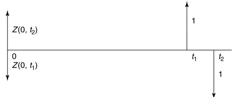
decreas-ing in t(equivalently, C(0, t) is increasing). Suppose Z(0,t1) < Z(0,t2) for some

t1< t2. Then the arbitrageur will buy a zero coupon bond for time t1, and

sell one for time t2, for an immediate income of Z(0,t2)—Z(0,t1) > 0. At time t1

they will receive 1 unit of currency from the bond they have bought, which

they could keep under their bed for all we care until time t2, when they

de-liver 1 in the bond they have sold.

What we have said so far assumes that such bonds do trade, with suf-ficient liquidity, and as a continuum i.e. a zero coupon bond exists for

every redemption date t. In fact, such bonds rarely trade in the market.

Rather what we need to do is impute such a continuum via a process known as bootstrapping.

It is more common for the market practitioner to think and work in terms of continuously compounded rates. The time 0 continuously

com-pounded risk free rate for maturity t, denoted r(t), is given by the

rela-tionship

C(0,t)=exp(r(t)t) (1)

Z(0,t)=exp(−r(t)t) (2)

r(t)= −1

t ln Z(0,t) (3)

In so-called normal markets, yield curves are upwardly sloping, with longer term interest rates being higher than short term. A yield curve which is downward sloping is called inverted. A yield curve with one or more turning points is called mixed. It is often stated that such mixed yield curves are signs of market illiquidity or instability. This is not the case. Supply and demand for the instruments that are used to bootstrap the curve may simply imply such shapes. One can, in a stable market with reasonable liquidity, observe a consistent mixed shape over long pe-riods of time.

Patrick S. Hagan

Chief Investment Office, JP Morgan 100 Wood Street London, EC2V 7AN, England,

e-mail: [email protected]

Graeme West

f(t)= −d

dtln(Z(t)) (7)

= d

dtr(t)t (8)

So f(t)=r(t)+r(t)t, so the forward rates will lie above the yield

curve when the yield curve is normal, and below the yield curve when it

is inverted. By integrating,1

r(t)t=

t

0

f(s)ds (9)

Z(t)=exp

−

t

0

f(s)ds

(10)

Also

riti−ri−1ti−1

ti−ti−1 = 1

ti−ti−1

ti

ti−1

f(s)ds (11)

which shows that the average of the instantaneous forward rate over any

of our intervals [ti−1,ti]is equal to the discrete forward rate for that

inter-val. Finally,

r(t)t=ri−1ti−1+

t

ti−1

f(s)ds, t∈[ti−1,ti] (12)

which is a crucial interpolation formula: given the forward function we easily find the risk free function.

2 Interpolation And Bootstrap Of Yield

Curves—Not Two Separate Processes

As has been mentioned, many interpolation methods for curve construc-tion are available. What needs to be stressed is that in the case of boot-strapping yield curves, the interpolation method is intimately connected to the bootstrap, as the bootstrap proceeds with incomplete information. This information is ‘completed’ (in a non unique way) using the interpo-lation scheme.

In Hagan and West [2006] we illustrated this point using swap curves; here we will make the same points focusing on a bond curve. Suppose we have a reasonably small set of bonds that we want to use to bootstrap the yield curve. (To decide which bonds to include can be a non-trivial exer-cise. Excluding too many runs the risk of disposing of market informa-tion which is actually meaningful, on the other hand, including too many could result in a yield curve which is implausible, with a multi-tude of turning points, or even a bootstrap algorithm which fails to con-verge.) Recall that we insist that whatever instruments are included will be priced perfectly by the curve.

Typically some rates at the short end of the curve will be known. For example, some zero-coupon bonds might trade which give us exact rates. In some markets, where there is insufficient liquidity at the short end, some inter-bank money market rates will be used.

Each bond and the curve must satisfy the following relationship:

^

The shape of the graph for Z(0, t) does not reflect the shape of the

yield curve in any obvious way. As already mentioned, the discount factor curve must be monotonically decreasing whether the yield curve is nor-mal, mixed or inverted. Nevertheless, many bootstrapping and interpola-tion algorithms for constructing yield curves miss this absolutely fundamental point.

Interestingly, there will be at least one class of yield curve where the

above argument for a decreasing Zfunction does not hold true— a real

(inflation linked) curve. Because the actual size of the cash payments that will occur are unknown (as they are determined by the evolution of a price index, which is unknown) the arbitrage argument presented

above does not hold. Thus, for a real curve the Zfunction is not

necessar-ily decreasing (and empirically this phenomenon does on occasion occur).

1.1 Forward rates

If we can borrow at a known rate at time 0 to date t1, and we can borrow

from t1to t2at a rate known and fixed at 0, then effectively we can

bor-row at a known rate at 0 until t2. Clearly

Z(0,t1)Z(0;t1,t2)=Z(0,t2) (4)

is the no arbitrage equation: Z(0;t1,t2)is the forward discount factor for

the period from t1to t2—it has to be this value at time 0 with the

infor-mation available at that time, to ensure no arbitrage.

The forward rate governing the period from t1 to t2, denoted

f(0;t1,t2)satisfies

exp(−f(0;t1,t2)(t2−t1))=Z(0;t1,t2)

Immediately, we see that forward rates are positive (and this is equiv-alent to the discount function decreasing). We have either of

f(0;t1,t2)= −

ln(Z(0,t2))−ln(Z(0,t1))

t2−t1

(5)

= r2t2−r1t1

t2−t1

(6)

Let the instantaneous forward rate for a tenor of t be denoted f(t), that

is, f(t)=lim∈↓0f(0;t,t+ ∈), for whichever t this limit exists. Clearly then

Z (0, t2)

Z (0, t1)

0

1

t1

1 t2

[A]=

n

i=0

piZ(0;tsettle,ti)

where

•

A

• tsettle is the date on which the cash is actually delivered for a pur-chased bond;

• p0,p1, . . . ,pnare the cash flows associated with a unit bond

(typical-ly p0=e₂c,pi= ₂c for 1≤i<nand pn=1+₂c where cis the annual

coupon and eis the cum-ex switch);

• t0,t1, . . . ,tnare the dates on which those cash flows occur.

On the left is the price of the bond trading in the market. On the right is the price of the bond as stripped from the yield curve. We rewrite this in the computationally more convenient form

[

A

n

i=0

piZ(0,ti) (13)

Suppose for the moment that the risk free rates (and hence the

dis-count factors) have been determined at t0,t1, . . . ,tn−1. Then we solve

Z(0,tn)easily as

Z(0,tn)=

1

pn

[

A

n−1

i=0

piZ(0,ti)

which is written in the form of risk-free rates rather than discount fac-tors as

rn=

1

tn

lnpn−ln

[

A

n−1

i=0

pie−riti

(14)

where the ti’s are now denominated in years and the relevant day-count

convention is being adhered to. Of course, in general, we do not know the earlier rates, neither exactly (because it is unlikely that any money

mar-ket instruments expire exactly at ti) nor even after some interpolation

(the rates for the smallest few ti might be available after interpolation,

but the later ones not at all). However, as in the case of swap curves, (14)

suggests an iterative solution algorithm: we guess rn, indeed other

ex-piry-date rates for other bonds, and take the rates already known from e.g. the money market, and insert these rates into our interpolation

algo-rithm. We then determine rsettle and r0,r1, . . . ,rn−1. Next, we insert these

rates into the right-hand side of (14) and solve for rn. We then take this

new guess for this bond, and for all the other bonds, and again apply the interpolation algorithm. We iterate this process. Even for fairly wild curves (such as can often be the case in South Africa) this iteration will reach a fixed point with accuracy of about 8 decimal places in 4 or 5 iter-ations. This then is our yield curve.

3 How To Compare Yield Curve

Interpolation Methodologies

In general, the interpolation problem is as follows: we have some data x

as a function of time, so we have τ1, τ2, . . . , τn and x1,x2, . . . ,xn known.

An interpolation method is one that constructs a continuous function

x(t) satisfying x(τi)=xi for i=1,2, . . . ,n. In our setting, the x values

might be risk free rates, forward rates, or some transformation of these— the log of rates, etc. Of course, many choices of interpolation function are

possible— according to the nature of the problem, one imposes

require-ments additional to continuity, such as differentiability, twice differen-tiability, conditions at the boundary, and so on.

The Lagrange polynomial is a polynomial of degree n−1which

pass-es through all the points, and of course this function is smooth. However, it is well known that this function is inadequate as an interpolator, as it demonstrates remarkable oscillatory behaviour.

The typical approach is to require that in each interval the function is described by some low dimensional polynomial, so the requirements of continuity and differentiability reduce to linear equations in the coeffi-cients, which are solved using standard linear algebraic techniques. The simplest example are where the polynomials are linear, and these meth-ods are surveyed in §4. However, these functions clearly will not be differ-entiable. Next, we try quadratics—however here we have a remarkable ‘zig-zag’ instability which we will discuss. So we move on to cubics—or even quartics—they overcome these already-mentioned difficulties, and we will see these in §5.

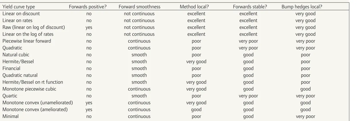
All of the interpolation methods considered in Hagan and West [2006] appear in the rows of Table 1.

We will restrict attention to the case where the number of inputs is reasonably small and so the bootstrapping algorithm is able to price the instruments exactly, and we restrict attention to those methods where the instruments are indeed always priced exactly.

The criteria to use in judging a curve construction and its interpola-tion method that we will consider are:

(a) In the case of yield curves, how good do the forward rates look? These are usually taken to be the 1m or 3m forward rates, but these are vir-tually the same as the instantaneous rates. We will want to have posi-tivity and continuity of the forwards.

It is required that forwards be positive to avoid arbitrage, while continuity is required as the pricing of interest sensitive instruments is sensitive to the stability of forward rates. As pointed out in McCulloch and Kochin [2000], ‘a discontinuous forward curve implies either implausible expectations about future short-term interest rates, or implausible expectations about holding period returns’. Thus, such an interpolation method should probably be avoided, es-pecially when pricing derivatives whose value is dependent upon such forward values.

Smoothness of the forward is desirable, but this should not be achieved at the expense of the other criteria mentioned here.

(b) How local is the interpolation method? If an input is changed, does the interpolation function only change nearby, with no or minor spill-over elsewhere, or can the changes elsewhere be material? (c) Are the forwards not only continuous, but also stable? We can

^

decree that the admissible hedging instruments are exactly those in-struments that were used to bootstrap the yield curve. Does most of the delta risk get assigned to the hedging instruments that have ma-turities close to the given tenors, or does a material amount leak into other regions of the curve?

We will now survey a handful of these methods, and highlight the issues that arise.

4 Linear Methods

4.1 Linear on rates

For ti−1<t<ti the interpolation formula is

r(t)= t−ti−1

ti−ti−1

ri+

ti−t

ti−ti−1

ri−1 (15)

Using (8) we get

f(t)= 2t−ti−1

ti−ti−1

ri+

ti−2t

ti−ti−1

ri−1 (16)

Of course fis undefined at the ti, as the function r(t)tis clearly not

dif-ferentiable there. Moreover, in the actual rate interpolation formula, by

the time treaches ti, the import of rt−1 has been reduced to zero—that

rate has ‘been forgotten’. But we clearly see that this is not the case for

the forward, so the left and right limits f(t+_i )and f(t_i−)are different—the

forward jumps. Furthermore, the choice of interpolation does not

pre-vent negative forward rates: suppose we have the (t, r) points (1y, 8%) and

(2y, 5%). Of course, this is a rather contrived economy: the one year inter-est rate is 8% and the one year forward rate in one year’s time is 2%. Nevertheless, it is an arbitrage free economy. But using linear interpola-tion the instantaneous forwards are negative from about 1.84 years on-wards.

4.2 Linear on the log of rates

Now for ti−1≤t≤tithe interpolation formula is

ln(r(t))= t−ti−1

ti−ti−1

ln(ri)+

ti−t

ti−ti−1 ln(ri−1)

which as a rate formula is

r(t)=r

t−ti−1 ti−ti−1

i r ti−t ti−ti−1

i−1 (17)

A simple objection to the above formula is that it does not allow neg-ative interest rates. Also, the same argument as before shows that the for-ward jumps at each node, and similar experimentation will provide an

example of a Zfunction which is not decreasing.

4.3 Linear on discount factors

Now for ti−1≤t≤tithe interpolation formula is

Z(t)= t−ti−1

ti−ti−1

Zi+

ti−t

ti−ti−1

Zi−1

which as a rate formula is

r(t)=−1

t ln

t−ti−1

ti−ti−1

e−riti+ ti−t

ti−ti−1

r−ri−1ti−1 ₍₁₈₎

Again, the forward jumps at each node, and the Zfunction may not be

decreasing.

4.4 Raw interpolation (linear on the log of discount

factors)

This method corresponds to piecewise constant forward curves. This method is very stable, is trivial to implement, and is usually the starting point for developing models of the yield curve. One can often find mis-takes in fancier methods by comparing the raw method with the more sophisticated method.

By definition, raw interpolation is the method which has constant

in-stantaneous forward rates on every interval ti−1<t<ti. From (11) we see

that that constant must be the discrete forward rate for the interval, so

f(t)= riti−ri−1ti−1

ti−ti−1 for ti−1<t<ti. Then from (12) we have that

r(t)t=ri−1ti−1+(t−ti−1)

riti−ri−1ti−1

ti−ti−1

By writing the above expression with a common denominator of ti−ti−1,

and simplifying, we get that the interpolation formula on that interval is

r(t)t= t−ti−1 ti−ti−1

riti+

ti−t

ti−ti−1

ri−1ti−1 (19)

which explains yet another choice of name for this method: ‘linear rt’;

the method is linear interpolation on the points riti. Since ±ritiis the

log-arithm of the capitalisation/discount factors, we see that calling this method ‘linear on the log of capitalisation factors’ or ‘linear on the log of discount factors’ is also merited.

This raw method is very attractive because with no effort whatsoever we have guaranteed that all instantaneous forwards are positive, because every instantaneous forward is equal to the discrete forward for the ‘par-ent’ interval. As we have seen, this is an achievement not to be sneezed at.

It is only at the points t1,t2, . . . ,tnthat the instantaneous forward is

un-defined, moreover, the function jumps at that point.

4.5 Piecewise linear forward

Having decided that the raw method is quite attractive, what happens if we try to remedy its only defect in the most obvious way? What we will do is that instead of the forwards being piecewise constant we will de-mand that they be a piecewise continuous linear function. What could be more natural than to simply ask to gently rotate the raw interpolants so that they are now not only piecewise linear, but continuous as well? Unfortunately, this very plausible requirement gives rise to at least two types of very unpleasant behaviour indeed. This is easily understood by

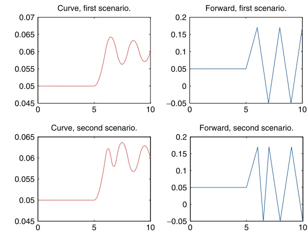
Firstly, suppose we have a curve with input zero coupon rates at every

year node, with a value of r(t)=5%for t=1,2, . . . ,5and r(t)=6%for

t=6,7, . . . ,10. We must have f(t)=r(1)for t≤1. In order to assure

con-tinuity, we see then we must have f(t)=r(i)for every i≤5. Now, the

dis-crete forward rate for [5, 6] is 11%. In order for the average of the

piecewise linear function fon the interval [5, 6] to be 11% we must have

that f(6)=17%. And now in turn, the discrete forward rate for [6, 7] is 6%

and so in order for the average of the piecewise linear function f on the

interval [6, 7] to be 6% we must have that f(7)= −5%. This zig-zag feature

continues recursively; see Figure 2. Note also the implausible shape of the actual yield curve itself.

Secondly, suppose now we include a new node, namely that

r(6.5)=6%. It is fairly intuitive that this imparts little new information2_.

Nevertheless, the bootstrapped curve changes dramatically. The ‘parity of the zig-zag’ is reversed. So we see that the localness of the method is exceptionally poor.

5 Splines

The various linear methods are the simplest examples of polynomial splines: a polynomial spline is a function which is piecewise in each in-terval a polynomial, with the coefficients arranged to ensure at least that the spline coincides with the input data (and so is continuous). In the lin-ear case that is all that one can do—the linlin-ear coefficients are now deter-mined. If the polynomials are of higher degree, we can use up the degrees of freedom by demanding other properties, such as differentia-bility, twice differentiadifferentia-bility, asymptotes at either end, etc.

The first thing we try is a quadratic spline.

5.1 Quadratic splines

To complete a quadratic spline of a function x, we desire coefficients

(ai,bi,ci) for 1≤i≤n−1. Given these coefficients, the function value at

any term τwill be

x(τ )=ai+bi(τ−τi)+ci(τ−τi)2 τi≤τ ≤τi+1 (20)

The constraints will be that the interpolating function indeed meets the given data (and hence is continuous) and the entire function is

differentiable. There are thus 3n−4constraints: n−1left hand function

values to be satisfied, n−1right hand function values to be satisfied,

and n−2 internal knots where differentiability needs to be satisfied.

However, there are 3n−3 unknowns. With one degree of freedom

re-maining, it makes sense to require that the left-hand derivative at τ_nbe

zero, so that the curve can be extrapolated with a horizontal asymptote.

Suppose we apply this method to the rates (so xi=ri). The forward

curves that are produced are very similar to the piecewise linear forward curves—the curve can have a ‘zig-zag’ appearance, and this zig-zag is sub-ject to the same parity of input considerations as before.

So, next we try a cubic spline.

5.2 Cubic splines

This time we desire coefficients (ai,bi,ci,di) for 1≤i≤n−1. Given these

coefficients, the function value at any term τwill be

x(τ )=ai+bi(τ−τi)+ci(τ−τi)2+di(τ−τi)3τi≤τ ≤τi+1 (21)

As before we have 3n−4 constraints, but this time there are 4n−4

unknown coefficients. There are several possible ways to proceed to find

another nconstraints. Here are the ones that we have seen:

• xi =ri. The function is required to be twice differentiable, which for

the same reason as previously adds another n−2 constraints. For

the final two constraints, the function is required to be linear at the

extremes i.e. the second derivative of the interpolator at τ₁and at τ_n

are zero. This is the so-called natural cubic spline.

• xi =ri. The function is again required to be twice differentiable; for

the final two constraints we have that the function is linear on the left and horizontal on the right. This is the so-called financial cubic spline Adams [2001].

• xi =riτi. The function is again required to be twice differentiable; for

the final two constraints we have that this function is linear on the right and quadratic on the left. This is the quadratic-natural spline proposed in McCulloch and Kochin [2000].

• xi =ri. The values of bifor 1<i<nare chosen to be the slope at τiof

the quadratic that passes through (τ_j,rj) for j=i−1,i,i+1. The

value of b1is chosen to be the slope at τ1of the quadratic that passes

through (τ_j,rj) for j=1,2,3; the value of bnis chosen likewise. This is

the Bessel method [de Boor, 1978, 2001, Chapter IV], although often somewhat irregularly called the Hermite method by software ven-dors.

0 5 10

0.045 0.05 0.055 0.06 0.065 0.07

Curve, first scenario.

0 5 10

−0.05 0 0.05 0.1 0.15 0.2

Forward, first scenario.

0 5 10

0.045 0.05 0.055 0.06 0.065

Curve, second scenario.

0 5 10

−0.05 0 0.05 0.1 0.15 0.2

Forward, second scenario.

^

• xi =riτi. Again, Bessel interpolation.

• Going one step further, quartic splines. According to Adams [2001] the quartic spline gives the smoothest interpolator of the forward curve. The spline can proceed on instantaneous forward rates, this

time there are 5n−5unknowns and 3 additional conditions at τ₁or

τ_nrequired. Although one must ask: when does one actually have a

set of instantaneous forwards as inputs for interpolation? Alternatively if we apply (9) then the inputs are risk free rates, and

the spline is of the form r(τ )=ai

τ +bi+ciτ+diτ

2_+e

iτ3+giτ4, with

6n−6unknowns and 4 additional conditions required.

• xi =ri. The monotone preserving cubic spline of Hyman [1983]. The

method specifies the values of bi for 1≤i≤n, in a way to be

dis-cussed in more detail shortly.

Significant problems can become apparent when using some of these methods. The spline is supposed to alleviate the problem of oscillation seen when fitting a single polynomial to a data set (the Lagrange polyno-mial), nevertheless, significant oscillatory behaviour can still be present. Furthermore, the various types of clamping we see with some of the methods above (clamping refers to imposing conditions at the

bound-aries τ₁ or τ_n) can compromise localness of the interpolator, sometimes

grossly. In fact, the iterative procedure from §2 often fails to converge for the quartic interpolation methods, and we exclude them from further analysis.

The method of Hyman is a method which attempts to address these problems. This method is quite different to the others; it is a local method—the interpolatory values are only determined by local behav-iour, not global behaviour. This method ensures that in regions of mo-notonicity of the inputs (so, three successive increasing or decreasing values) the interpolating function preserves this property; similarly if the data has a minimum/maximum then the output interpolator will have a minimum/maximum at the node.

6 Monotone Convex

Many of the ideas of the method of Hyman will now have a natural devel-opment—the monotone convex method was developed to resolve the only remaining deficiency of Hyman [1983]. Very simply, none of the methods mentioned so far are aware that they are trying to solve a financial prob-lem—indeed, the breeding ground for these methods is typically engi-neering or physics. As such, there is no mechanism which ensures that the forward rates generated by the method are positive, and some simple experimentation will uncover a set of inputs to a yield curve which give some negative forward rates under all of the methods mentioned here, as seen in Hagan and West [2006]. Thus, in introducing the monotone con-vex method, we use the ideas of Hyman [1983], but explicitly ensure that the continuous forward rates are positive (whenever the discrete forward rates are themselves positive).

The point of view taken in the monotone convex method is that the inputs are (or can be manipulated to be) discrete forwards belonging to intervals; the interpolation is not performed on the interest rate curve it-self. We may have actual discrete forwards—FRA rates. On the other hand

if we have interest rates r1,r2, . . . ,rn for periods τ1, τ2, . . . , τn then the

first thing we do is calculate fd

i =

riτi−ri−1τi−1

τi−τi−1 for 1≤i≤n,r0=0. (Here we

also check that these are all positive, and so conclude that the curve is legal i.e. arbitrage free (except in those few cases where forward rates may be negative). As an interpolation algorithm the monotone convex method will now bootstrap a forward curve, and then if required recover the continuum of risk free rates using (12).

One rather simple observation is that all of the spline methods we

saw in §5 fail in forward extrapolation beyond the interval [τ1, τn]. Clearly

if the interpolation is on rates then we will apply horizonal extrapolation

to the rate outside of that interval: r(τ )=r1for τ < τ1 and r(τ )=rnfor

τ > τn. So far so good. What happens to the forward rates? Perhaps

sur-prisingly we cannot apply the same extrapolation rule to the forwards, in

fact, we need to set f(τ )=r1for τ < τ1and f(τ )=rnfor τ > τn—consider

(8). This makes it almost certain that the forward curve has a material

discontinuity at τ1, and probably one at τn too (the latter will be less

se-vere as the curve, either by design or by nature, probably has a horizontal

asymptote as τ ↑τn).

In order to avoid this pathology, we now have terms 0=τ0, τ1, . . . , τn

and the generic interval for consideration is [τi−1, τi]. A ‘short rate’

(in-stantaneous) rate may be provided, if not, the algorithm will model one. Usually the shortest rate that might be input will be an overnight rate, if it is provided, the algorithm here simply has some ‘overkill’—there will be an overnight rate and an instantaneous short rate—but it need not be modified.

fd

i is the discrete rate which ‘belongs’ to the entire interval [τi−1, τi]; it

would be a mistake to model that rate as being the instantaneous rate at

τi. Rather, we begin by assigning it to the midpoint of the interval, and

then modelling the instantaneous rate at τi. as being on the straight line

that joins the adjacent midpoints. Let this rate f(τi)be denoted fi. This

ex-plains (22). In (23) and (24) the values f0=f(0)and fn=f(τn)are selected

so that f(0)=0=f(τn). Thus

fi=

τ_i−τ_i−1 τ_i+1−τ_i−1f

d i+1+

τ_i+1−τ_i τ_i+1−τ_i−1f

d

i, for i=1,2, . . . ,n−1 (22)

f0=f1d−12(f1−f

d

1) (23)

fn=fnd−12(fn−1−f

d

n) (24)

Note that if the discrete forward rates are positive then so are the fi for

i=1,2, . . . ,n−1.

We now seek an interpolatory function f defined on [0, τn] for

f0,f1, . . . ,fn that satisfies the conditions below (in some sense, they are

arranged in decreasing order of necessity).

(i) 1

τi−τi−1 τi

τi−1f(t)dt=f

d

i , so the discrete forward is recovered by the

curve, as in (11).

(ii) f is positive.

(iii) f is continuous.

(iv) If fd

i−1<fid<fid+1 then f(τ ) is increasing on [τi−1, τi], and if

fd

i−1>fid>fid+1then f(τ )is decreasing on [τi−1, τi].

Let us first normalise things, so we seek a function gdefined on [0, 1]

g(x)=f(τ_i−1+(τ_i−τ_i−1)x)−fd

i . (25)

Before proceeding, let us give a sketch of how we will proceed. We will

choose gto be piecewise quadratic in such a way that (i) is satisfied by

construction. Of course, gis continuous, so (iii) is satisfied. As a

quadrat-ic, it is easy to perform an analysis of where the minimum or maximum

occurs, and we thereby are able to apply some modifications to gto

en-sure that (iv) is satisfied, while ensuring (i) and (iii) are still satisfied.

Also, we see a posteriori that if the values of fi had satisfied certain

constraints, then (ii) would have been satisfied. So, the algorithm will be

to construct (22), (23) and (24), then modify the fi to satisfy those

con-straints, then construct the quadratics, and then modify those quadrat-ics. Finally,

f(τ )=g

_τ−τ i−1 τi−τi−1

+fd

i . (26)

Thus, the current choices of fiare provisional; we might make some

adjustments in order to guarantee the positivity of the interpolating

function f.

Here follow the details. We have only three pieces of information about

g: g(0)=fi−1−fid,g(1)=fi−fid, and 1

0 g(x)dx=0. We postulate a

func-tional form g(x)=K+Lx+Mx2_{, having 3 equations in 3 unknowns we get}

⎡

⎣11 01 01

1 1

2 1 3

⎤ ⎦

⎡ ⎣KL

M

⎤ ⎦₌

⎡ ⎣gg((01))

0

⎤

⎦, and easily solve to find that

g(x)=g(0)[1−4x+3x2_{]+g(1)[−2x+3x}2_{] (27)}

Note that by (22) that (iv) is equivalent to requiring that if fi−1<fid<fi

then f(τ )is increasing on [τ_i−1, τ_i], while if fi−1>fid>fi then f(τ )is

de-creasing on [τ_i−1, τ_i]. This is equivalent to requiring that if g(0) and g(1)

are of opposite sign then gis monotone.

Now

g(x)=g(0)(−4+6x)+g(1)(−2+6x)

g(0)= −4g(0)−2g(1)

g(1)=2g(0)+4g(1)

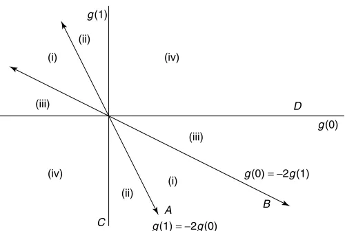
g being a quadratic it is now easy to determine, simply by inspecting

g(0)and g(1), the behaviour of g on [0, 1]. The cases where g(0)=0and

g(1)=0 are crucial; these correspond to g(1)= −2g(0) and

g(0)= −2g(1)respectively. These two lines divide the g(0)/g(1) plane into

eight sectors. We seek to modify the definition of g on each sector, taking care that on the boundary of any two sectors, the formulae from those

two sectors actually coincide (to preserve continuity). In actual fact the treatment for every diametrically opposite pair of sectors is the same, so we really have four cases to consider, as follows (refer Figure 4):

(i) In these sectors g(0) and g(1) are of opposite signs and g(0)and g(1)

are of the same sign, so gis monotone, and does not need to be

mod-ified.

(ii) In these sectors g(0) and g(1) are also of opposite sign, but g(0)and

g(1)are of opposite sign, so gis currently not monotone, but needs

to be adjusted to be so. Furthermore, the formula for (i) and for (ii)

need to agree on the boundary Ato ensure continuity.

(iii) The situation here is the same as in the previous case. Now the

for-mula for (i) and for (iii) need to agree on the boundary Bto ensure

continuity.

(iv) In these sectors g(0) and g(1) are of the same sign so at first it appears

that gdoes not need to be modified. Unfortunately this is not the

case: modification will be needed to ensure that the formula for (ii)

and (iv) agree on Cand (iii) and (iv) agree on D.

The origin is a special case: if g(0)=0=g(1)then g(x)=0for all x, and

fd i−1=f

d i =f

d

i+1, and we put f(τ )=f

d

i for τ∈[τi−1, τi].

So we proceed as follows:

(i) As already mentioned g does not need to be modified. Note that

on A we have g(x)=g(0)(1−3x2_{) and on B we have g(x)=g(0)}

(1−3x+3 2x2).

(ii) A simple solution is to insert a flat segment, which changes to a

quadratic at exactly the right moment to ensure that ₀1g(x)dx=0.

So we take

g(x)=

_{g(0) for 0≤x≤η}

g(0)+(g(1)−g(0))

x−η

1−η 2

for η <x≤1 (28)

η=1+3 g(0)

g(1)−g(0)=

g(1)+2g(0)

g(1)−g(0) (29)

Note that η−→0as g(1)−→ −2g(0), so the interpolation formula

reduces to g(x)=g(0)(1−3x2_{)at A, as required.}

0 x = 0

τ =τi–1

x = 0

τ =τi

g(0)

g(1)

Figure 3: The function g.

g (0) g (1)

g (1) _{= −}2g (0)

g (0) = −2g (1) (i)

(ii)

(iv)

(iii)

(ii) (iv)

(iii) (i)

C

A B

D

^

(iii) Here again we insert a flat segment. So we take

g(x)=

g(1)+(g(0)−g(1))

η−x

η 2

for 0<x< η

g(1) for η≤x<1 (30)

η=3 g(1)

g(1)−g(0) (31)

Note that η−→1 as g(1)−→ −1₂g(0), so the interpolation formula

reduces to g(x)=g(0)(1−3x+3

2x2)at B, as required.

(iv) We want a formula that reduces in form to that defined in (ii) as we

approach C, and to that defined in (iii) as we approach D. This

sug-gests

g(x)=

⎧ ⎨ ⎩

A+(g(0)−A)

η−x

η 2

for 0<x< η

A+(g(1)−A)

x−η

1−η 2

for η <x<1

(32)

where A=0when g(1)=0- so the first line satisfies (iii)) and A=0

when g(0)=0(so the second line satisfies (ii). Straightforward

calcu-lus gives

1

0

g(x)dx=2

3A+

η

3g(0)+

1−η

3 g(1)

and so

A= −1

2[ηg(0)+(1−η)g(1)]

A simple choice satisfying the various requirements is

η= g(1)

g(1)+g(0) (33)

A= − g(0)g(1)

g(0)+g(1) (34)

6.1 Ensuring positivity

Suppose we wish to guarantee that the interpolatory function fis

every-where positive.

Clearly from the formula (26) it suffices to ensure that g(x) >−fd

i for x∈[0,1]. Now g(0)=fi−1−fid>−fidand g(1)=fi−fid>−fidsince fi−1,fi

are positive. Thus the inequality is satisfied at the endpoints of the

inter-val. Now, in regions (i), (ii) and (iii), gis monotone, so those regions are

fine.

In region (iv) gis not monotone. gis positive at the endpoints and has

a minimum of A(as in (34)) at the x-value η(as in (33)). So, it now suffices

to prove that _gg₍₀(0₎₊)g_g(1₍₁)₎ <fd

i. This is the case if fi−1,fi<3fid. To see this, note

that then 0<g(0),g(1) <2fd

i and the result follows, since if 0<y,z<2a

then y+_yzz= 1_z+1_y > 1 2a +

1 2a =

1

a and so

yz y+z >a.

We choose the slightly stricter condition fi−1,fi<2fid. Thus, our

algo-rithm is

(1) Determine the fd

i from the input data.

(2) Define fifor i=0,1, . . ., nas in (22), (23) and (24).

(3) If f is required to be everywhere positive, then collar f0 between 0

and 2fd

1, for i=1,2, . . . ,n−1 collar fi between 0 and 2min(fid,fid+1),

and collar fnbetween 0 and 2fnd. If fis not required to be everywhere

positive, simply omit this step.

(4) Construct gwith regard to which of the four sectors we are in.

(5) Define f as in (26).

(6) If required recover ras in (12). Integration formulae are easily

estab-lished as the functions forms of gare straightforward.

Pseudo-code for this recipe is provided in an Appendix. Working code for this interpolation scheme is available from the second author’s website.

6.2 Amelioration

In Hagan and West [2006] an enhancement of this method is considered where the curve is ameliorated (smoothed). This is achieved by making the interpolation method slightly less local i.e. by using as inputs not only neighbouring information but also information which is two nodes away.

7 Hedging

We can now ask the question: how do we use the instruments which have been used in our bootstrap to hedge other instruments? In general

0 0.5 1

−1 0 1 −1 0 1 −1 0 1 −1 0 1 −1 0 1 −1 0 1 −1 0 1 −1 0 1 −1 0 1 −1 0 1 −1 0 1 −1 0 1 −1 0 1 −1 0 1 −1 0 1 −1 0 1 −1 0 1 −1 0 1 −1 0 1 −1 0 1

0 0.5 1 0 0.5 1 0 0.5 1

0 0.5 1 0 0.5 1 0 0.5 1 0 0.5 1

0 0.5 1 0 0.5 1 0 0.5 1 0 0.5 1

0 0.5 1 0 0.5 1 0 0.5 1 0 0.5 1

0 0.5 1 0 0.5 1 0 0.5 1 0 0.5 1

3m 3x6 6x9 9x12 12x15 15x18 2y 3y 4y 5y 6y 7y 8y 9y 10y 15y 20y 25y 30y 1

0.5 0 0.5 1

Hedging under waves.

3m 3x6 6x9 9x12 12x15 15x18 2y 3y 4y 5y 6y 7y 8y 9y 10y 15y 20y 25y 30y −2

−1 0 1 2

Hedging under forward triangles.

3m 3x6 6x9 9x12 12x15 15x18 2y 3y 4y 5y 6y 7y 8y 9y 10y 15y 20y 25y 30y 0.2

0 0.2 0.4 0.6 0.8

Hedging under forward boxes.

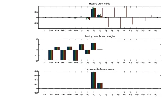
Figure 6: The obvious superiority of using forward boxes to determine hedge portfolios: not only is the hedge portfolio simple and intuitive, but the portfolio composition is practically invariant under the interpolation method.

the trader will have a portfolio of other, more complicated instru-ments, and will want to hedge them against yield curve moves by using liquidly traded instruments (which, in general, should exactly be those instruments which were used to bootstrap the original curve). For sim-plicity, we will assume that these instruments are indeed available for hedging, and the risky instrument to be hedged is nothing more com-plicated that another vanilla swap: for example, one with term which is not one of the bootstrap terms, is a forward starting swap, or is a stubbed swap.

Suppose initially that, with n instruments being used in our

boot-strap, there are exactly nyield curve movements that we wish to hedge

against. It is easy to see that we can construct a perfect hedge. First one

calculates the square matrix Pwhere Pij is the change in price of the jth

bootstrapping instrument under the ith _{curve. Next we calculate the}

change in value of our risk instrument under the ith _{curve to form a}

column vector V. The quantity of the ith _{bootstrapping instrument}

re-quired for the perfect replication is the quantity Qiwhere Qis the

solu-tion to the matrix equasolu-tion PQ =V. Assuming for the moment that Pis

invertible, we find the solution.

Of course, in reality, the set of possible yield curve movements is far,

far greater. What one wants to do then is find a set of n yield curve

changes whose moves are somehow representative. Some methods have been suggested as follows:

• Perturbing the curve: creation of bumps. In bumping, we form new

curves indexed by i: to create the ith_{curve one bumps up the i}th_input

rate by say 1 basis point, and bootstraps the curve again.

• Perturbing the forward curve with triangles. One approach is to

again form new curves, again indexed by i: the ith _{curve has the}

original forward curve incremented by a triangle, with left hand

endpoint at ti−1, fixed height say one basis point and apex at ti, and

right hand endpoint at ti+1. (The first and last triangle will in fact

be right angled, with their apex at the first and last time points respectively.)

• Perturbing the forward curve with boxes. In boxes: the ith _{curve has}

the original forward curve incremented by a rectangle, with left

hand endpoint at ti−1and right hand endpoint at ti, and fixed height

say one basis point. Such a perturbation curve corresponds exactly

with what we get from bumping, if one of the inputs is a ti−1×tiFRA

rate, we bump this rate, and we use the raw interpolation method.

^

terms - the inputs to the bootstrap do not necessarily correspond to these nodes.

In either case we have (an automated or user defined) set of dates

t1,t2, . . . ,tnwhich will be the basis for our waves, where the triangles are

defined as above.

Some obvious ideas which are just as obviously rejected are to form corresponding perturbations to the yield curve itself - such curves will

not be arbitrage free (the derived Zfunction will not be decreasing).

As an example, consider a 51m swap, where (for simplicity, and in-deed, in some markets, such as the second author’s domestic market) both fixed and floating payments in swaps occur every 3 months. Thus our swap lies between the 4 and 5 year swap, which let us assume are in-puts to the curve.

The type of results we get are in Figure 6. The very plausible and popular bump method performs adequately for many methods, but some methods - for example, the minimal method - can be rejected out of hand if bumping is to be used. Furthermore, for all of the cubic splining methods, there is hedge leakage of varying degrees. Perturbing with triangles can be rejected out of hand as a method - in-deed, the pathology that occurs here is akin to the pathology that aris-es when one usaris-es the piecewise forward linear method of bootstrap: adding or removing an input to the bootstrap will reverse the sign of the hedge quantities before the input in question. Anyway, to have these magnitudes in the hedge portfolio is simply absurd. Perturbing with boxes is the method of choice, but unfortunately does not enable us to distinguish between the quality of the different interpolation methods.

8 Conclusion

The comparison of the methods we analyse in Hagan and West [2006] appears in Table 1.

It is our opinion that the new method derived in Hagan and West [2006], namely monotone convex (in particular, the unameliorated ver-sion) should be the method of choice for interpolation. To the best of our knowledge this is the only published method where simultaneously

(1) all input instruments to the bootstrap are exactly reproduced as out-puts of the bootstrap,

(2) the instantaneous forward curve is guaranteed to be positive if the inputs allow it (in particular, the curve is arbitrage free), and (3) the instantaneous forward curve is typically continuous.

In addition, as bonuses

(4) the method is local i.e. changes in inputs at a certain location do not affect in any way the value of the curve at other locations.

(5) the forwards are stable i.e. as inputs change, the instantaneous for-wards change more or less proportionately.

(6) hedges constructed by perturbations of this curve are reasonable and stable.

In Hagan and West [2006] we have reviewed many interpolation meth-ods available and have introduced a couple of new methmeth-ods. In the final analysis, the choice of which method to use will always be subjective, and needs to be decided on a case by case basis. But we hope to have provided some warning flags about many of the methods, and have outlined sev-eral qualitative and quantitative criteria for making the selection on which method to use.

Yield curve type Forwards positive? Forward smoothness Method local? Forwards stable? Bump hedges local?

Linear on discount no not continuous excellent excellent very good

Linear on rates no not continuous excellent excellent very good

Raw (linear on log of discount) yes not continuous excellent excellent very good

Linear on the log of rates no not continuous excellent excellent very good

Piecewise linear forward no continuous poor very poor very poor

Quadratic no continuous poor very poor very poor

Natural cubic no smooth poor good poor

Hermite/Bessel no smooth very good good poor

Financial no smooth poor good poor

Quadratic natural no smooth poor good poor

Hermite/Bessel on rt function no smooth very good good poor

Monotone piecewise cubic no continuous very good good good

Quartic no smooth poor very poor very poor

Monotone convex (unameliorated) yes continuous very good good good

Monotone convex (ameliorated) yes continuous good good good

Minimal no continuous poor good very poor

Pseudo Code For Monotone Convex

Interpolation

First the estimates for f0,f1, . . . ,fn. This implementation assumes that

it is required that the output curve is everywhere positive. Various arrays

FOOTNOTES & REFERENCES

1.We have r(s)s+C=f(s)ds,sor(t)t=[r(s)s]t

0=

t

0f(s)ds.

2.It would be wrong to say that there is no new information; that would be the case under linear interpolation of rates, but not necessarily here.

3.Strictly speaking, we are defining functions gi, each corresponding to the interval

[τ_i−1, τ_i]. As the giare constructed one at a time, we suppress the subscript.

[1] Ken Adams. Smooth interpolation of zero curves. Algo Research Quarterly,

4(1/2):11—22, 2001.

[2] Carl de Boor. A Practical Guide to Splines: Revised Edition,volume 27 of Applied Mathematical Sciences.Springer-Verlag New York Inc., 1978, 2001.

[3] Patrick S. Hagan and Graeme West. Interpolation methods for curve construction.

Applied Mathematical Finance,13 (2):89—129, 2006.

[4] James M. Hyman. Accurate monotonicity preserving cubic interpolation. SIAM Journal on Scientific and Statistical Computing,4(4):645—654, 1983.

[5] J. Huston McCulloch and Levis A. Kochin. The inflation premium implicit in the US real and nominal term structures of interest rates. Technical Report 12, Ohio State University Economics Department, 2000. URL http://www.econ.ohio-state.edu/jhm/jhm.html.

[6] Ricardo Rebonato. Interest-Rate Option Models.John Wiley and Sons Ltd, second edi-tion, 1998.

have already been dimensioned, the raw data inputs have already been provided, and it has been specified with the boolean variable

‘InputsareForwards’ where those inputs are rates r1,r2, . . . ,rnor discrete

forwards fd

1,f2d, . . . ,fnd. Further, a ‘collar’ and ‘min’ utility functions

are used (not shown). Of course, collar(a,b,c)=max(a,min(b,c)).

Having found the estimates for f0,f1, . . . ,fn, we can find the value of

f(τ )for any τ. The key function here is ‘LastIndex’, which determines

the unique value of ifor which τ ∈[τ_i, τ_i+1). Extrapolation is as in

W

Working code for this interpolation scheme, with proper dimensioning of all arrays and code for all the missing functions, is available from the