Nonlinear forecasts of fo F2: variation of model predictive accuracy over time

Annales

Geophysicae

Nonlinear forecasts of foF2: variation of model predictive accuracy

over time

A. H. Y. Chan and P. S. Cannon*

Centre for RF Propagation and Atmospheric Research, QinetiQ, Malvern, UK

*_{Also at the Department of Electronic and Electrical Engineering, University of Bath, UK}

Received: 1 October 2001 – Revised: 26 February 2002 – Accepted: 13 March 2002

Abstract. A nonlinear technique employing radial basis function neural networks (RBF-NNs) has been applied to the short-term forecasting of the ionospheric F2-layer criti-cal frequency, foF2. The accuracy of the model forecasts at a northern mid-latitude location over long periods is assessed, and is found to degrade with time. The results highlight the need for the retraining and re-optimization of neural network models on a regular basis to cope with changes in the statis-tical properties of geophysical data sets. Periodic retraining and re-optimization of the models resulted in a reduction of the model predictive error by∼0.1 MHz per six months. A detailed examination of error metrics is also presented to il-lustrate the difficulties encountered in evaluating the perfor-mance of various prediction/forecasting techniques.

Key words. Ionosphere (ionospheric disturbances; model-ing and forecastmodel-ing) – Radio science (nonlinear phenomena)

1 Introduction

Variations in the solar, magnetospheric, and ionospheric characteristics can affect a variety of ground-based and space-borne technological systems (e.g. Hargreaves, 1995; Feynman and Gabriel, 2000). Disturbances in the ionosphere can degrade radio propagation and satellite communications; solar flares can cause positional errors of several kilometers in ground-based navigation systems, and the Global Position-ing System (GPS) can be affected by variations in electron density in the ionosphere. Magnetic storms can induce cur-rents in long-distance pipelines and cable networks. Magne-tospheric particles and solar proton flares can affect space-craft by causing radiation and structural damage. Conse-quently, predictions of geomagnetic storms have a significant bearing upon the operation of a number of services (Joselyn, 1995).

The importance of nonlinear behavior within the solar-terrestrial environment has been demonstrated by Baker et Correspondence to: A. H. Y. Chan ([email protected])

al. (1990), and attempts have been made in modeling the nonlinear dynamics in geomagnetic activity (e.g. Klimas et al., 1992; Vassiliadis et al., 1995). However, due to the incomplete understanding of the physics of the Sun-magnetosphere-ionosphere coupled system, many theoretical and empirical models often fail to accurately predict iono-spheric disturbances and geomagnetic storm events (Jose-lyn, 1995). An attractive alternative approach would be to adopt knowledge-independent modeling techniques that can cope with the problems of noise and non-contiguity typically found in geophysical data sets.

A number of studies have investigated the application of neural networks (NNs) to geophysical prediction problems (e.g. Lundstedt, 1992; Williscroft and Poole, 1996; Wu and Lundstedt, 1997; Francis et al., 1997, 2000; Cander et al., 1998; Wintoft and Cander, 2000). In this work, we shall refer to short-term (e.g. 1-hour ahead) predictions as fore-casts, in order to distinguish these from the more commonly referred-to longer-term (e.g. monthly median) predictions. Many of the above studies have used multiple inputs. For example, Lundstedt (1992) used solar section boundary data, coronal mass ejection data, solar wind and coronal hole data to train neural networks for the prediction of a number of effects including geomagnetic induced currents, while Wu and Lundstedt (1997) used solar wind andDst data as in-puts to neural networks for the forecasting of geomagnetic storms. Williscroft and Poole (1996) predicted daily and monthly noon values of the ionospheric parameter foF2 at Grahamstown, South Africa, using seasonal time informa-tion, solar and magnetic activities as input data. Cander et al. (1998) presented a 1-hour ahead forecasting technique for foF2 and the total electron content (TEC) using input data which included foF2/TEC, a daily sunspot number andDst index. Wintoft and Cander (2000) used foF2 data, together with magnetic activity indexAE, time-of-day and seasonal information to forecast foF2 values for 1 to 24 h ahead. The above types of models are more commonly known as cross-prediction models.

persistence model for 1-month ahead predictions. Such a comparison with simple recurrence and persistence models is a minimum prerequisite of any rigorous assessment of new forecasting algorithms, and without it, performance claims with respect to new algorithms are rendered meaningless.

An assessment of the true value of space weather predic-tion schemes is, however, more complicated than a simple (albeit valuable) comparison with recurrence and persistence models. The space weather environment is nonstationary over a number of time scales, ranging from periods of days to 11 years or more. However, typical data sets are shorter than 11 years, and even when these long data sets are available, it may not be possible to undertake the necessary matrix opera-tions on the data set as a whole (due to limited computing re-sources). Consequently, the neural network models and their associated error statistics usually presented are quite specific to a particular epoch. This was illustrated forcefully when a re-optimized version of the Francis et al. (2000) 1-hour ahead forecasting model was incorporated into our real-time fore-casting system – the Ionospheric Forefore-casting Demonstrator, IFD (http://www.cpar.qinetiq.com). It soon became clear that the predictive capability of the IFD was degrading with time. In this paper, we describe a number of methods for assessing the long-term performance of NN models, and illustrate how the predictive accuracy of a NN model can be maintained in a non-stationary environment.

2 Analysis approach

Solar-terrestrial data sets are typically very noisy. The Time Series Analysis Routines (TSAR) described by Smith et al. (1998) employ novel and robust methods that can cope with the problems of noise and data dropouts. The detailed math-ematical theory behind the TSAR software can be found in Smith et al. (1998). Here, we shall give a brief summary of the Radial Basis Function Neural Network (RBF-NN) model used in this study.

2.1 Principal component analysis

The use of principal component analysis (PCA) in the pre-processing of the time series allows for the separation of the signal and noise subspaces, and improves the performance

data points (Xn,Yn), wheren= 1. . . N, andN =total num-ber of data points in the time series, to a model of the form

Y = f (X). The RBF-NN offers one approach to the solu-tion of this problem, and has the advantage over the more commonly used Multi-Layer Perceptron (MLP) techniques of being able to find a globally optimum solution to a time series prediction problem in a single pass training process that determines the appropriate model weights (Broomhead and Lowe, 1988). (MLPs can only produce locally optimum solutions through an iterative training process.)

In the RBF approach, f (Xn) is assumed to be a linearly weighted sum of radially symmetric functions ofX, such that

f Xn

= N

X

i=1

ωiϕi |Xn−ci |

, (1)

whereωi are the weights of the functionsϕi, andci are the centers of radial symmetry.

The set of model parameters, including window length and number of centers, is optimized to give the best solution to the functionf (Xn)such that the errorEis minimized

E=

N

X

n=1 h

f Xn

−Yn

i2

. (2)

The effectiveness of the prediction model can be quan-tified in terms of the normalized root-mean-squared error (NRMSE), which is essentially the root-mean-squared error (RMSE) divided by the standard deviation, σ, of the input data NRMSE = v u u u u u u t N P n=1 h

f Xn−Yn

i2

N

P

n=1 h

Xn−X

i2

=RMSE

σ , (3)

whereXis the mean value ofXn,n=1. . . N. A NRMSE of zero indicates a perfect prediction, while a NRMSE of unity indicates that the model is no more effective than taking the mean of the data.

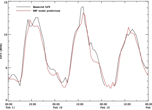
Fig. 1. Measured foF2 and 1-hour ahead forecasts during a storm event in February 2000. The gap in the mea-sured foF2 time series represent missing data.

the NRMSE was found to be 0.26, representing an improve-ment of∼35% and 42% over the reference persistence and 24-hour recurrence models, respectively.

3 Data analysis

3.1 Data description

For this study, hourly foF2 measurements from the UK ionosonde station at Chilton (51.6◦_{N, 358.7}◦_{E) from June} 1995 to October 2000 are used. Measurements at the Chilton station started in the mid-1990’s, and after an initial settling-in period, the percentage of misssettling-ing data posettling-ints per year fell to∼4% in 1997, a value which has since been maintained.

As is typical in many geophysical data sets, the time se-ries used in this study contains many data dropouts (e.g. as-sociated with instrument failure, and data values which fall outside the accepted range of the foF2 parameter). These discontinuities in the data time series pose a significant ob-stacle for prospective nonlinear prediction schemes, which generally require continuous data. A nonlinear interpolation technique, which minimizes the effects of interpolation upon any given modeling process, has been developed by Francis et al. (2001) to deal with data gaps in the time series. For 1-hour ahead forecasts, this has been shown to provide an overall improvement of 2.3% and 3.8% over the 24-hour re-currence and persistence interpolation schemes, respectively. This nonlinear interpolation technique, however, is compu-tationally and time intensive, and as a result, has not been utilized in this study. Instead, missing data points are inter-polated using the 24-hour recurrence values.

3.2 Model description and test error analysis

A number of optimized NN forecasting models were gen-erated using the data time series of foF2 from the Chilton ionosonde station. The optimization process involves adjust-ing the input vector window length and centers, as discussed in the previous section. Each model contains 1.5 years’ worth of data, of which 75% of the data points available were used to train and optimize the model, and the remaining 25% were used to test the model’s predictive accuracy on unseen data. The remainder of the period of available data (up to October 2000) was then used to evaluate the long-term performance of the model.

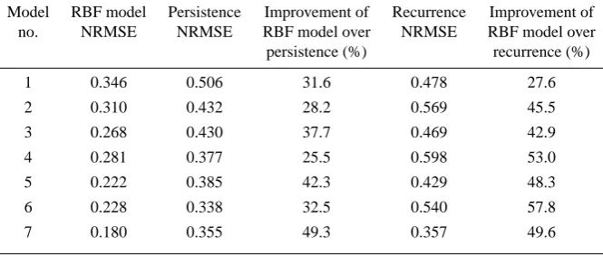
The data periods used for each model, the data character-istics, such as the mean and standard deviation, σ, of the input data, and the percentage of missing data, are detailed in Table 1. The data are characterized by improving qual-ity, a higher mean value, and increased variability as time progressed. Also included in the table are the model test er-rors. As an indication of the effectiveness of the nonlinear modeling routines against the more common linear model-ing techniques, the model test errors (based on the last 25% of the input data time series) are compared with that from the reference persistence and recurrence models, which assume that the data pointYn+1will be the same asYnandYn−23,

re-spectively (Table 2). The considerable improvements of the RBF-NN models over persistence predictions can be seen to range from approximately 25 to 50%, while improvements over 24-hour recurrence predictions are between ∼28 and 58%.

3.3 Long-term model error analysis

7 1 Jul 98–31 Dec 99 Jan 00 4.08 6.11 2.01 0.180

Table 2. Comparison of RBF model normalized root-mean-squared errors (NRMSE) with persistence and 24-hour recurrence model NRMSE

Model RBF model Persistence Improvement of Recurrence Improvement of no. NRMSE NRMSE RBF model over NRMSE RBF model over persistence (%) recurrence (%)

1 0.346 0.506 31.6 0.478 27.6

2 0.310 0.432 28.2 0.569 45.5

3 0.268 0.430 37.7 0.469 42.9

4 0.281 0.377 25.5 0.598 53.0

5 0.222 0.385 42.3 0.429 48.3

6 0.228 0.338 32.5 0.540 57.8

7 0.180 0.355 49.3 0.357 49.6

normalized root-mean-squared errors (NRMSE) for 1-hour ahead forecasts for the series of models from January 1997 to October 2000 are shown in Fig. 2. Each point repre-sents a monthly averaged value (calculated by summing over all available data points in the month and then dividing by the total number of data points), and each curve starts after the previously described test period has ended (see Table 1). Immediately apparent is the degradation which occurs with time, and the benefit accrued from periodic retraining and re-optimizing of the neural network models. Model retraining every year, and most beneficially every 6 months, is neces-sary.

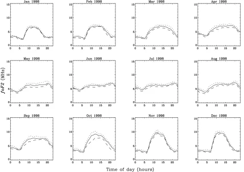
It can also be clearly seen that the NRMSEs are smaller in winter than in summer, indicating that the RBF-NN mod-els perform better during winter. To examine the reason for this difference, we need to look at the variation in the foF2 time series over the course of one year, an example of which is shown in Fig. 3. During the winter months, the foF2 data exhibits a clear diurnal variation, whereas the summer varia-tion is unclear, with the peak-to-peak variavaria-tion being smaller and almost noise-like. As can be seen from Eq. (3), if all other factors remain unchanged, then the smaller variation in the summer data will result in a higher NRMSE. From

the perspective of the neural network developer, our model is, therefore, more successful in making the winter forecasts. However, while the NRMSE provides a useful measure of the model’s success, the normalization obscures the absolute error associated with the forecast. For systems assessment, this might be more important.

Fig. 2. Normalized root-mean-squared errors for 1-hour ahead forecasts of foF2 from January 1997 to October 2000.

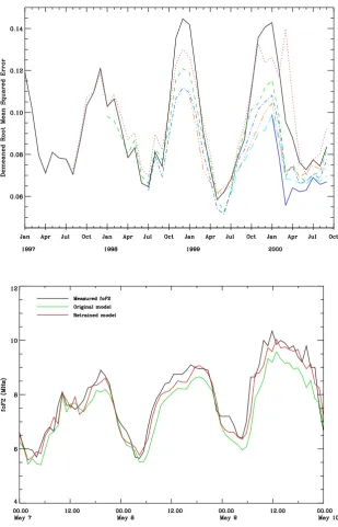
Fig. 4. Root-mean-squared errors for 1-hour ahead forecasts of foF2 from Jan-uary 1997 to October 2000 (Legend as in Fig. 2).

Fig. 5. Monthly mean foF2 values from July 1995 to October 2000.

Also seen in Fig. 4 is the general increasing trend in the RMSE. The time period over which the forecasts are made is during an ascending phase of the solar cycle, as can be seen in Fig. 5, which shows the monthly mean foF2 values from July 1995 to October 2000. To compensate for this in-creasing trend in the mean foF2 data, we have demeaned the root-mean-squared errors by dividing by the monthly mean of the input data (Fig. 6). The annual variation in RMSE still remains.

3.4 Retraining versus re-optimizing

We have shown in the previous section the benefits of peri-odic re-optimization of neural network models to cope with

Fig. 6. Demeaned root-mean-squared errors for 1-hour ahead forecasts of foF2 from January 1997 to October 2000 (Legend as in Fig. 2).

Fig. 7. Measured foF2 and 1-hour ahead forecasts from original and re-trained models for the time period 7–9 May 2000.

In the absence of adequate resources, we have investigated an alternative approach to improving the model predictive ac-curacy on a new data set. The approach simply retrains the neural network model to obtain new weights while still using previously optimized window length and centers. This ap-proach saves considerable computer processing time, in that a “new” model can be generated in a matter of hours rather than weeks. Figure 7 shows the actual foF2 time series, to-gether with the comparison of nonlinear forecasts performed using an out-of-date model, and that using a retrained model. Even though not fully optimized, the retrained model shows clear improvements over the out-of-date model. Thus, in the absence of adequate processing time, simply retraining the model rather than re-optimizing can prove to be a useful

option to improve model forecasts.

4 Conclusions

vide a meaningful measure of the model’s success; the lat-ter is a necessary requirement for understanding the utility of these prediction techniques in practical applications. Clearly, no one metric tells the complete story, and it is incumbent on all forecasters to provide a realistic range of error metrics. Acknowledgements. This work was carried out by the United King-dom Defence Evaluation and Research Agency (DERA) / QinetiQ Ltd., and was funded by the United Kingdom Ministry of Defence TG9/RO6 Corporate Research Programme.

The data time series used in this study were obtained from the World Data Center (WDC) archive at the Rutherford Appleton Lab-oratory (RAL) (http://www.wdc.rl.ac.uk/wdcc1/ionosondes/data archive.html).

Topical Editor M. Lester thanks A. Stocker and L. Cander for their help in evaluating this paper.

References

Baker, D. N., Klimas, A. J., McPherron, R. L., and Buchner, J.: The evolution from weak to strong geomagnetic activity: An in-terpretation in terms of deterministic chaos, Geophys. Res. Lett., 17, 41–44, 1990.

Broomhead, D. S. and Lowe, D.: Multivariable functional inter-polation and adaptive networks, Complex Systems, 2, 321–355, 1988.

D. S.: Prediction of the hourly ionospheric parameter foF2 using a novel nonlinear interpolation technique to cope with missing data points, J. Geophys. Res., 106, A12, 30 077–30 083, 2001. Hargreaves, J. K.: The solar-terrestrial environment, Cambridge

University Press, pp. 420, 1995.

Joselyn, J. A.: Geomagnetic activity forecasting: The state of the art, Rev. Geophys., 33, 3, 383–401, 1995.

Klimas, A. J., Baker, D. N., Roberts, D. A., Fairfield, D. H., and Buchner, J.: A nonlinear dynamic analogue model of geomag-netic activity, J. Geophys. Res., 97, A8, 12 253–12 266, 1992. Lundstedt, H., Neural networks and predictions of solar terrestrial

effects, Planet. Sp. Sci., 40, 4, 457–464, 1992.

Smith, R. J. K., Brown, A. G., and Francis, N. M.: Time Se-ries Analysis Routines (TSAR) V4.0 User Manual, DERA, DERA/CIS(CIS2)/WP98048, 1998.

Vassiliadis, D., Klimas, A. J., Baker, D. N., and Roberts, D. A.: A description of the solar wind-magnetosphere coupling based on nonlinear filters, J. Geophys. Res., 100, A3, 3495–3512, 1995. Williscroft, L. A. and Poole, A. W. V.: Neural Networks, foF2,

sunspot number and magnetic activity, Geophys. Res. Lett., 23, 24, 3659–3662, 1996.

Wintoft, P. and Cander, L. R.: Ionospheric foF2 storm forecasting using neural networks, Phys. Chem. Earth C, 25, 4, 267–273, 2000.