Least-squares gradient calculation from multi-point observations of scalar and vector fields: methodology and applications with Cluster in the plasmasphere

Ann. Geophys., 25, 971–987, 2007 www.ann-geophys.net/25/971/2007/ © European Geosciences Union 2007

Annales

Geophysicae

Least-squares gradient calculation from multi-point observations of

scalar and vector fields: methodology and applications with Cluster

in the plasmasphere

J. De Keyser1, F. Darrouzet1, M. W. Dunlop2, and P. M. E. D´ecr´eau3

1_{Belgian Institute for Space Aeronomy (BIRA-IASB), Ringlaan 3, 1180 Brussels, Belgium} 2_{Rutherford Appleton Laboratory (RAL), Chilton, Didcot, Oxfordshire OX11 0QX, UK}

3_{Laboratoire de Physique et Chimie de l’Environnement (LPCE/CNRS), 3A Avenue de la Recherche Scientifique, 45071} Orl´eans Cedex 02, France

Received: 26 September 2006 – Revised: 30 March 2007 – Accepted: 4 April 2007 – Published: 8 May 2007

Abstract. This paper describes a general-purpose algorithm for computing the gradients in space and time of a scalar field, a vector field, or a divergence-free vector field, from in situ measurements by one or more spacecraft. The algo-rithm provides total error estimates on the computed gradi-ent, including the effects of measurement errors, the errors due to a lack of spatio-temporal homogeneity, and errors due to small-scale fluctuations. It also has the ability to diagnose the conditioning of the problem. Optimal use is made of the data, in terms of exploiting the maximum amount of infor-mation relative to the uncertainty on the data, by solving the problem in a weighted least-squares sense. The method is illustrated using Cluster magnetic field and electron density data to compute various gradients during a traversal of the inner magnetosphere. In particular, Cluster is shown to cross azimuthal density structure, and the existence of field-aligned currents in the plasmasphere is demonstrated.

Keywords. Magnetospheric physics (Magnetospheric con-figuration and dynamics; Plasmasphere; Instruments and techniques)

1 Introduction

This paper deals with the computation of gradients of phys-ical quantities (scalar or vector fields) that are measured in situ at different times and positions. This topic has gained importance in the context of recent magnetospheric multi-spacecraft missions, in particular the Cluster mission con-sisting of four identical spacecraft, flying in formation. The rationale behind this mission is the idea that exactly four si-multaneous measurements are needed to determine the three spatial gradient components, at least if the four spacecraft are not coplanar. Methods to do so have been developed Correspondence to: J. De Keyser

([email protected])

x

1

x

2

l

u

l

1

u

sc

3

sc

2

sc

1

x

Fig. 1. The least-squares gradient algorithm uses data acquired in a set of points in space-time, represented

here as a 2-dimensional space (x1,

x2). In this example, the data are obtained along the trajectories of three

spacecraft (red dots on the dotted lines), although that does not matter for the method. The homogeneity

condition is expressed by associating with each data point an error that grows with the distance from

x0, the

point where the gradient is computed. This distance, however, is measured in a frame (

l

l

rotated and scaled relative to the original frame. Points on the ellipse with semi-axes

l

and

l

are assigned a unit

distance. Points inside the ellipse (dark shaded area) correspond to smaller distances and therefore a smaller

error. Points outside that ellipse (lightly shaded region) will have a larger error so that they are less relevant,

thus reflecting the homogeneity condition. Points outside the shaded regions are considered irrelevant.

a set of points in space-time, represented here as a 2-dimensional space (x₁,x₂). In this example, the data are obtained along the tra-jectories of three spacecraft (red dots on the dotted lines), although that does not matter for the method. The homogeneity condition is expressed by associating with each data point an error that grows with the distance fromx0, the point where the gradient is com-puted. This distance, however, is measured in a frame (l1u1,l2u2) that may be rotated and scaled relative to the original frame. Points on the ellipse with semi-axesl1andl2are assigned a unit distance. Points inside the ellipse (dark shaded area) correspond to smaller distances and therefore a smaller error. Points outside that ellipse (lightly shaded region) will have a larger error so that they are less relevant, thus reflecting the homogeneity condition. Points outside the shaded regions are considered irrelevant.

1997, 2001; Trotignon et al., 2003) because of their abso-lute calibration (Darrouzet et al., 2006b). (5) Additional er-rors arise due to the lack of synchronization of the spacecraft clocks, the nonzero duration over which data are gathered, and the uncertainties in the spacecraft positions. The impact of these errors may be hard to quantify, especially because they may not be statistically independent. Such errors tend to be relevant for short time scales and small separations only.

This paper describes an alternative way to determine the gradient obtained by relaxing the requirement of simultane-ity of the observations. This is achieved by formulating the concepts of temporal and spatial homogeneity in a more gen-eral way. By using all observations in a region of space-time over which the spatial and temporal gradients are essentially constant over prescribed length and time scales, an overde-termined system of equations is obtained from which the gra-dient can be computed in a least-squares sense. In principle,

data from an arbitrary number of spacecraft can be exploited. It is possible to attempt to compute gradients on length and time scales that match the physical scales of interest. In any given practical situation the method will find out whether such gradients can actually be computed with the available data. For in situ measurements by the Cluster spacecraft in a medium that is at rest, for instance, the scales along the spacecraft orbit will usually be limited by the time resolution of the data, while the scales perpendicular to the velocity will be dictated by the orbital separations. Proper error estimates are derived that account for the measurement errors, for the errors due to the fact that the gradient is not constant over the region in which measurements are available, and for the effect of small-scale structures and perturbing wave fields. It is also possible to take into account geometrical and spatio-temporal constraints.

In Sects. 2–5, the method is presented in a formal math-ematical way. We use linear algebra techniques (such as eigen-decomposition and singular value decomposition) and therefore adopt the standard linear algebra notation: Bold lower-case symbols represent vectors, bold upper-case sym-bols are matrices, other symsym-bols denote scalars. Sections 6–8 illustrate the application of the method for scalar fields, for vector fields, and for divergence-free vector fields with Clus-ter examples for a pass through the inner magnetosphere.

2 The problem for scalar fields

One or more spacecraft sample a scalar field f (x, t ) at positions and times xi=[xi;yi;zi;ti], i=1, . . . , N, in 4-dimensional space-time. The case of vector fields is dis-cussed later. The measurementsfi have known error vari-ancesδf_meas,i2 . Data intercalibration removes all systematic errors (we disregard clock synchronization and spacecraft position errors).

The gradient ∇_xtf=[∂f/∂x;∂f/∂y;∂f/∂z;∂f/∂t] at a pointx0 can be computed by combining all measurements made inside a region in which the gradient does not change appreciably. This region is the “homogeneity domain”. Its size is determined by physical considerations. It can be de-scribed by a 4-dimensional ellipsoid, that is, by four mutually orthonormal directionsuj and the corresponding scales lj, specifying the axes of the hyperellipsoid. This is illustrated in Fig. 1 by means of an analogy in 2-dimensional space. In this example, the points (red dots) are obtained along the tra-jectories of three spacecraft (dotted lines), although that does not matter for the method. The points inside the homogeneity domain (represented by the dark shaded ellipse) can safely be used to compute the gradient inx0. Rather than accepting points inside the homogeneity domain for the computation and rejecting points outside, we will use a more gradual ap-proach. With each data point, we will associate an error that grows with the distance fromx0. This distance, however, is measured in a frame (l1u1,l2u2) that may be rotated and

J. De Keyser et al.: Least-squares gradient calculation 973 scaled relative to the original (x1,x2) frame. This frame will

be called theβ-frame, and the unit coordinate vectors of this frame are exactly the semi-axes of the elliptical homogeneity domain. Points on the border of the homogeneity domain are assigned a unit distance. Points inside the ellipse correspond to smaller distances and therefore a smaller error. Points far-ther outside that ellipse have a larger error so that they are of progressively diminishing relevance, thus reflecting the ho-mogeneity condition.

The transformation xβ=Px, where P=(UL)−1 with orthonormal matrix U=[. . .uj. . .] and diagonal matrix

L=diag(lj) (this notation means: the diagonal ma-trix with the lj on the diagonal) represents the tran-sition from the original frame to the new frame, de-noted by superscript β, in which the homogeneity do-main is the unit hypersphere. The corresponding gra-dient operator is ∇β_xt=P−1>∇xt=LU>∇xt. The dis-tance measure that is needed to express the homogene-ity condition assigns to each vector x a length or norm

kxk_β= √

xβ>_xβ₌√_x>_UL−2_U>_x.

Homogeneity considerations in time are often sep-arable from spatial homogeneity. One of the uj must then be [0;0;0;1]. If the time scale is lt=τ and if the three spatial homogeneity scales are lx=ly=lz=ξ, the transformation is simply a rescaling

P=diag([1/ξ,1/ξ,1/ξ,1/τ]). Theβ-norm of a given vec-tor x then is kxk_β=

q

(x/ lx)2+(y/ ly)2+(z/ lz)2+(t / lt)2. We will refer to this particular case as the standard isotropic homogeneity case.

If f satisfies the appropriate analyticity conditions near

x0, it can be locally approximated by a Taylor expansion. With1xi=xi−x0, and denoting the function value and the gradient atx0byf0and∇xtf0, this becomes

fi =f0+1xi>∇xtf0+ri, (1) where the residual isri=O(k1xik2). This leads to a system ofNequations forf0and∇xtf0, i.e.,M=5 unknowns:

r =f0+1X>∇xtf0−f=f0+1Xβ>∇xtβf0−f=0 (2) where1X=[. . .1xi. . .]groups all relative positions andf denotes all measurements. The homogeneity domain can usually be chosen big enough so thatNM: The system is overdetermined and can never be satisfied exactly. However, the gradient can be computed in a least-squares sense (min-imization ofr>_{r). Expressing this system in the β-frame} (the dimensionless form) is preferable from the numerical point of view (since all system matrix elements then are of order unity). Although system (2) is usually overdetermined, it may still be ill-conditioned. Such ill-conditioning can of-ten be avoided by adding a priori knowledge in the form of constraints. In the case of Cluster it may become possible to compute gradients with only three, two, or even a single spacecraft, depending on the number of constraints. We will not use such constraints in the present paper, but Appendix A explains how they can be incorporated.

3 Approximation errors

In order to obtain the gradient, we approximate the scalar fieldf, with all its space-time variations, by a local linear approximation. There are two aspects to this approximation: The function might have variations at scales smaller than the specified homogeneity scale (this variability usually cannot be evaluated completely from the measurements, so a sta-tistical approach is needed to estimate its effect), and there is also the curvature off at the homogeneity scale itself, which is why the linear approximation is only valid inside the homogeneity domain. Both contribute to the total “ap-proximation error”; the small-scale errors are the “fluctuation errors” and the errors due to the linear approximation are the “curvature errors”. We will therefore write the scalar field as f=fhs+δfls+δfss, the sum of the linear fieldfhsat the ho-mogeneity scale (i.e. the linear approximation), a deviation δflsdue to variations at larger scales, and a small-scale field δfss.

3.1 Structure at large scales

Structure at large scales (1xβ=k1xk_β≥1) is properly repre-sented by the Taylor expansion of Eq. (1). With the constant fcindicating how muchfchanges over the homogeneity do-main due to the higher-order terms in the expansion (function curvature), the curvature error is estimated as

δf_ls2(1xi)≤fc2(1x β i )

4_,

so that the linear approximation is valid when1xβ_i<1 but not much beyond that. The curvature error is completely deter-mined by the homogeneity conditions through theβ-norm. The user must specify the value offcbased on physical con-siderations. This may not be trivial, as will be discussed in Sect. 6 and in the Conclusions. Note that the value offcis linked to the homogeneity lengths: halving the homogeneity lengths is equivalent to multiplyingfc by a factor of four. In principle, the curvature errors at the various sampling po-sitions are not statistically independent, but since nothing is known about them a priori, their cross-correlations are ig-nored here. This is justified even more so because, as ex-plained in Sect. 5, only little weight will be given to data points far fromx0for which the cross-correlations would be large.

this corresponds to the classical spatial gradient computation (Harvey, 1998; Chanteur, 1998; Chanteur and Harvey, 1998). 3.2 Structure at small scales

Small-scale structure is often present, for instance in the form of small-amplitude waves or turbulence. Small-scale per-turbations are usually under-sampled, so their influence on gradient precision must be characterized with a stochastic model.

Theδfss(x)can be thought of as the superposition of in-dividual perturbations, each with length scalesλj along mu-tually orthogonal directions, which we take to be the homo-geneity directionsuj for the sake of simplicity, and with am-plitudeδfssλ(λ,x):

δfss(x)= Z

λ

δfssλ(λ,x) dλ.

Let the population of perturbations δfss be character-ized by typical length scales λˆ. We can then in-troduce a new reference frame γ, similar to frame β but with different axis scaling, which leads to a norm

kxk_γ= √

x>_U3−2_U>_{x where 3=diag(λ}ˆ_{). Restricting} ourselves to distributions that are isotropic in γ-space and assuming that the perturbation amplitudes do not vary appreciably over the homogeneity domain, one has

h(δfssλ(λ,x))2i=δfλ2(λγ) everywhere, with λγ=kλkγ and where the acute brackets identify the expected value for the population of perturbations. Because of the local-ity of the perturbations,hδfssλ(λ,xi)δfssλ(λ,xj)i≈δfλ2(λγ) when1x_ijγ=kxj−xikγλγ and zero when1xijγλγ. Ap-pendix B computes that, for a distribution with perturbation strengthδf_λ2(λγ)decreasing exponentially, the covariances are

hδfss(xi)δfss(xj)i =f∗2e−1x

γ ij_,

with f∗2 the total perturbation variance. The cross-correlation is large between nearby points and vanishes as their distance exceeds the perturbation length. Better mod-els are possible if the type of perturbation (e.g. a particular wave mode) is known a priori. In such cases it would be best to compute the gradients of several wave field components simultaneously, coupled through the wave relations.

4 The problem for vector fields

The gradients of the individual components of a vector field can be obtained by treating each component individually as a separate scalar field under the simplifying assumption that the curvature errors are not correlated (or that one does not know a priori how) and that the small-scale perturbations for the different components are uncorrelated as well (which is not really true if they are due to a particular wave mode). Dif-ferent homogeneity parameters for each of the components

(differentuj,lj,fc,λjˆ ,f∗) could be used. Here, the discus-sion is limited to the case of identical values. The number of unknowns at each point isM=3×5=15. For divergence-free vector fields (such as the magnetic field) the gradients of the vector components must be computed simultaneously, subject to the constraint that the divergence vanishes, so that M=14.

Computing the curl and the divergence of the vector field poses an additional difficulty. As the divergence and each of the components of the curl are sums of terms of the same or-der of magnitude, but possibly with opposite sign, the relative error on the result can be larger than the relative errors on the individual gradient components, which themselves are dif-ferences of similar values and have a significant uncertainty.

5 Solving the overdetermined system

The overdetermined system (2) expressingN measurements of a scalar field (the number of equations) can be written as

r =Aq−f =0, (3)

withA=1,1Xβ>

and whereq=[f0;∇β_xtf0]is the vector ofM=5 unknowns. The total error onfias used in the gradi-ent computation atx0isδf_i2=(δfmeas,i)2+fc2(1x

β

i )4+f∗2, in which the terms represent the independent contribu-tions of measurement error, curvature error and fluctua-tion error. In addition, there are the cross-correlations δf_ij2=f∗2e−1x

γ

ij_{. These estimates give theN×N correlation}

matrixCf=hδf δf>i, which is real, symmetric, and positive definite. It is strongly diagonal dominant if theδfmeas,i and fcare large, iff∗is small, or if theλjˆ are small. AsN may be large, significant computing time and storage savings can be achieved by setting the off-diagonalsδf_ij2 to zero if1x_ijγ is above an appropriately chosen limit, thus ignoring small cross-correlations (typically e−1x

γ

ij_<10−4_).

The eigen-decomposition Cf=W>D2W is computed, whereWcontains the orthonormal eigen-vectors and where the non-negative eigen-values, which are denoted byd_i2, con-stitute the diagonal matrixD2_=diag(d2

i). This is trivial ifCf is diagonal, i.e., when we do not consider small-scale fluc-tuations. Applying operatorWon the left to the vectorsr,

f, andAqin the overdetermined system (3), the errors on the transformed residuals are now statistically independent, so that thei-th equation represents an individual piece of in-formation corresponding to a covarianced_i2. A further oper-ation byD−1on the left normalizes the residuals so that they all have unit variance, by dividing each by its error estimate. The resulting weighted system is

˜

r = ˜_Aq−f˜=0, (4)

J. De Keyser et al.: Least-squares gradient calculation 975 method minimizes r˜>_{r˜ so that equations with less}

rele-vant information (d_i2 large) will hardly play a role. Large measurement errors and short-scale fluctuations reduce the weights, and data points outside the homogeneity domain have such important curvature errors that their weight is neg-ligible, thus ensuring that the information used for comput-ing the gradient comes from within the homogeneity domain. Consider the situation depicted in Fig. 1. Spacecraft 2 passes nearx0and has three points inside the homogeneity domain (the dark shaded ellipse), the middle of which carries only measurement and fluctuation errors while the curvature error is small there. Spacecraft 1 does not have any point inside the homogeneity domain. Nevertheless, its data points just outside the homogeneity domain (in the light shaded region) will also appear in the overdetermined system. As their cur-vature errors are larger, their weights will be smaller. They therefore contribute only a limited amount of information in the computation of the gradient.

The least-squares solution is obtained by formally solving the overdetermined system as

q=(A˜>A˜)−1A˜>f˜.

In practice, computing A˜>_A˜ _{(an M×M symmetric} posi-tive semidefinite matrix) is avoided because it implies sums with many terms and therefore a potential loss of precision. The standard method is to compute a decompositionA˜=QR, where Q is a unitary N×M matrix and R is an M×M upper triangular matrix with the so-called economy-size QR-algorithm. One can then easily computeA˜>A˜=_R>_R. This symmetricM×M matrix can be inverted by comput-ing its scomput-ingular value decompositionA˜>_A˜_=V>_S2_{V, where}

S=diag(sj)are the singular values andVis unitary, so that

q=V>S−2VA˜>f˜. (5)

The correlation of errors on the result is Cq=(A˜>A˜)−1, from which the errors on the result can be estimated as

δq=pdiag(Cq) by ignoring the cross-correlations be-tween the solution components. From q=[f0;∇β_xtf0]

and δq=[δf0;δ(∇βxtf0)], the gradient and the er-ror estimates are found as ∇xtf0=UL−1∇β_xtf0 and δ(∇_xtf0)=UL−1δ(∇βxtf0).

As can be seen from Eq. (5), the solution is obtained by applying the transformationV>_S−2_{Vto the weighted data}

˜

A>_f˜_{. SinceVis unitary, the conditioning of the problem is} completely determined by the singular valuessj. If a singu-lar value is small, the propagation of errors in the associated direction is important. For spatial gradient computations us-ing simultaneous data from the four Cluster spacecraft, the concepts of planarity and elongation of the spacecraft tetra-hedron have been used as a diagnostic for the well-posedness of the problem (Robert et al., 1998a,b), which have the ad-vantage of being easily visualized. The singular values, how-ever, provide an abstract but general diagnostic that works

for an arbitrary number of spacecraft and in the presence of constraints (Appendix A). We therefore define the condition number

cond=min j s

2 j/max

j s 2

j. (6)

Even when the problem is close to singular (condition num-ber small) the method produces a valid result, but the error estimates on the result (or, at least, on some of its compo-nents) will be large. As results with too large errorbars are useless, computations with cond<10−5are ignored.

The technique described here is based on an unconstrained approximation off. If the scalar field is strictly positive, it is best to apply the technique to_f¯_{=logf, withδf}¯_=δf/f.

The results are transformed back using∇xtf=ef¯∇xtf¯and δ(∇xtf )=ef¯[δ(∇xtf )¯+δf¯∇xtf¯].

When computing the gradients of the three components of a vector fieldB, supplemented by the condition∇·B=0, the overdetermined system is



  

11Xβ> ₀

N×5 0N×5

0N×5 11Xβ> 0N×5

0N×5 0N×5 11Xβ>

0u1>/ l1 0u2>/ l2 0u3>/ l3 

   

       

Bx0 ∇β_xtBx0

By0 ∇β_xtBy0

Bz0 ∇β_xtBz0



        =



  

Bx,N×1

By,N×1

Bz,N×1 0



  

with a 3×3 block-diagonal coefficient matrix supplemented by the zero-divergence condition.

In the particular situation in which all data have been ac-quired simultaneously, the coefficients of the time derivatives are all zero and no information about the time variations can be extracted. The corresponding unknowns can be removed from the system, so thatM=4 for the gradient of a scalar field,M=12 for a vector field, andM=11 for a divergence-free vector field.

6 Gradients of a scalar field

(b)

ne

[cm

−3

]

06:00 06:30 07:00 07:30 08:00 08:30 09:00 09:30 10:00 10:30 11:00 101

102

10 9 8 7 6 5 4.53 5 6 7 8 9 10 (a)

|B| [nT]

250 300 350 400 450

Fig. 2. Cluster observations during a pass through the inner magnetosphere on August 7, 2003, from 06:00–

11:00 UT, with perigee around 08:02 UT: (a) magnetic field strength|B|obtained from the FGM magnetometer,

and (b) electron densitynecomputed from the plasma frequency as identified by the WHISPER instrument.

The spacecraft separation distances were200×400×1000 kmin the GSEX,Y,Zdirections near perigee.

|B|reaches a local minimum andnea maximum around perigee (C1 - black, C2 - red, C3 - green, C4 - blue).

The bottom scale gives theL-shell position of the center of the Cluster tetrahedron (forL <10, elsewhereL

cannot be determined accurately).

24

Fig. 2. Cluster observations during a pass through the inner magnetosphere on 7 August 2003, from 06:00–11:00 UT, with perigee around 08:02 UT: (a) magnetic field strength|B|obtained from the FGM magnetometer, and (b) electron densityne computed from the plasma frequency as identified by the WHISPER instrument. The spacecraft separation distances were 200×400×1000 km in the GSEX,Y,Z

directions near perigee.|B|reaches a local minimum andnea maximum around perigee (C1 – black, C2 – red, C3 – green, C4 – blue). The bottom scale gives theL-shell position of the center of the Cluster tetrahedron (forL<10, elsewhereLcannot be determined accurately).

situation in which the plasmapause typically is located rather close to Earth). The plasma encountered near perigee (be-tween 07:40 and 08:40 UT) is of plasmaspheric origin, as in-dicated by the Cluster plasma spectrometers. CIS/CODIF on Cluster 4, for instance, detects He+and O+. The spectrom-eters also indicate corotating flow of a few km/s, although the measurements are not very precise since the instruments miss a major fraction of the cold plasma distributions due to spacecraft potential effects. The|B|profiles are smooth with minor variations at the begin and the end of the pass, when the spacecraft are outside the plasmasphere and sample higherL-values at higher magnetic latitudes, and whereneis low. FGM is very precise and well calibrated. Spin-averaged magnetic field data (4 s time resolution) are used here. The measurement error on the components is 0.1 nT while the un-certainty on|B|is 0.15 nT (<0.05 %). These data appear to allow an accurate gradient determination since the magnetic field values registered by the four spacecraft at any given time differ by up to 10 nT, larger than the measurement er-rors. The measurement error onfpis the 163 Hz discretiza-tion error (half of the frequency resoludiscretiza-tion of WHISPER). Additional errors due to the possible misidentification of the plasma frequency line in the WHISPER spectrograms have been kept to a minimum as the algorithms for plasma fre-quency detection have matured (Trotignon et al., 2001, 2003, 2006; Rauch et al., 2006). The relation between densityne

and plasma frequencyfpis ne[cm−3] =(fp[kHz]/9.0)2,

from which δne/ne=2δfp/fp. The peak density is almost 70 cm−3 with an error of 0.3 cm−3. The relative error is smallest for these high densities, typically 0.4 %, and in-creases up to 20 % for lower densities near the detection limit.

J. De Keyser et al.: Least-squares gradient calculation 977

(h)

10 9 8 7 6 5 4.53 5 6 7 8 9 10

(a) (a) (a)

(g)

∂

|B|

/

∂

t

[nT/s]

06:00 06:30 07:00 07:30 08:00 08:30 09:00 09:30 10:00 10:30 11:00 −0.02

0 0.02 (f)

|

∇

|B|| [nT/m]

0.00000 0.00005 0.00010 (e)

cond(

∇

|B|)

10−15 10−10 10−5 100 (d)

Neff

0 10 20 (c)

N

0 50 100 150 (b)

Seff

0.7 0.75 0.8 0.85 (a)

|B| [nT]

250 300 350 400 450

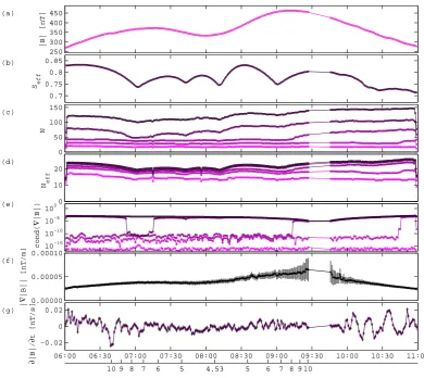
Fig. 3. Computation of∇xt|B|every60 swith isotropic homogeneity domain (see text). (a) magnetic field

strength|B|at the moving center of the homogeneity domain; (b) effective scale factorSeff; (c) number of

equationsNin the overdetermined system, where each curve refers to a thresholdσk, with darker color shade as

σkincreases; (d) effective number of equationsNeff; (e) problem condition number for eachσk; (f) magnitude

of the spatial gradient|∇|B||, with growing error bars and gap in the computed gradient due to spacecraft

coplanarity; (f) temporal gradient∂|B|/∂t. The bottom scale gives theL-shell position of the center of the

Cluster tetrahedron.

25

Fig. 3. Computation of∇_xt|B|every 60 s with isotropic homogeneity domain (see text). (a) magnetic field strength|B|at the moving center of the homogeneity domain; (b) effective scale factorSeff; (c) number of equationsNin the overdetermined system, where each curve refers to a thresholdσk, with darker color shade asσk increases; (d) effective number of equationsNeff; (e) problem condition number for each

σk; (f) magnitude of the spatial gradient|∇|B||, with growing error bars and gap in the computed gradient due to spacecraft coplanarity; (g) temporal gradient∂|B|/∂t. The bottom scale gives theL-shell position of the center of the Cluster tetrahedron.

can be included in the weighted system for determining the gradient at a given point. As the weights of most points are negligible, however, it is computationally more efficient to include only those points with a relative variance satisfying ρi =δfi2/min

j δf 2 j < σk,

where theσkis a series of increasing threshold values. In the example sketched in Fig. 1 this threshold corresponds to the outer ellipse: All points included in the computation form a set that is larger than the homogeneity domain (assuming that the measurement and fluctuation errors for all points are the same, otherwise there exists no simple geometrical rep-resentation). In practice, we use 5 logarithmically spaced valuesσk from 2 up to 100, for each of which the gradient is computed. The gradient computation is thus repeated with the outer ellipse being progressively expanded. The result is most precise for the largest threshold (largestN). Solving the problem for allσkallows us to assess whether the largest

threshold is too low (a better result could be obtained) or un-necessarily large (computationally inefficient). Figure 3 il-lustrates the computation of∇_xt|B|. It has been determined every 60 s. The magnetic field strength at the moving center of the homogeneity domain is a spatio-temporal average of the observed values (panel a). In order to find the physical scales of this averaging process, note that the region from which the weighted least-squares method will take most of its information (where homogeneity-scale error≤ measure-ment error+fluctuation error) has a diameter or effective scale sizeDj in thej-th homogeneity direction that can be computed from

(Dj/lj)4=16(δfmeas2 +f∗2)/fc2=Seff4 ,

(g)

06:00 06:30 07:00 07:30 08:00 08:30 09:00 09:30 10:00 10:30 11:00 −0.02

0 0.02 (f)

∂

|B|

/

∂

t

[nT/s]

−0.02 0 0.02 (e)

−0.02 0 0.02 (d)

0.00000 0.00005 0.00010 (c)

|

∇

|B|| [nT/m]

0.00000 0.00005 0.00010 (b)

0.00000 0.00005 0.00010

10 9 8 7 6 5 4.53 5 6 7 8 9 10 (a)

cond(

∇

|B|)

10−4 10−2

Fig. 4. Computation of∇xt|B|with isotropic homogeneity domain (red), anisotropic domain (green), and

anisotropic domain with small-scale fluctuations (blue) (see text). (a) condition number; (b–d) magnitude of

spatial gradient|∇|B||; (e–f) temporal gradient∂|B|/∂t. The bottom scale gives theL-shell position of the

center of the Cluster tetrahedron.

26

Fig. 4. Computation of∇xt|B|with isotropic homogeneity domain (red), anisotropic domain (green), and anisotropic domain with small-scale fluctuations (blue) (see text). (a) condition number; (b–d) magnitude of spatial gradient|∇|B||; (e–g) temporal gradient∂|B|/∂t. The bottom scale gives theL-shell position of the center of the Cluster tetrahedron.

is that Seff becomes smaller as fc becomes larger, reflect-ing the equivalence between small homogeneity scales with a smallfc on the one hand, and larger homogeneity scales with a larger fc on the other hand. The number of equa-tionsNactually used to compute the gradient (panel c, each curve refers to aσk) increases withσk. A measure for the amount of information used is the effective number of equa-tionsNeff=P

i1/ρi, which is the sum of the inverse relative variances of the corresponding equations, so that Neff≤N (panel d). For ever larger σk, Neff increases, but the rel-ative gain decreases as the added equations have progres-sively lower weights. The convergence of theNeff-curves in-dicates that maxkσk=100 is well-chosen. Figure 3e presents an overview of the condition number as defined by Eq. (6). For lowσk(Nsmall, not necessarily using data from the four spacecraft) the problem is almost singular (cond∼10−16), but for largerσkthe condition number becomes very reasonable, typically 10−3. It remains below 10−5 in the time interval 09:30–09:45 UT, so that the gradient cannot be sensibly com-puted there. The growing errorbars on the magnitude of the

spatial gradient, |∇|B||, correspond to this ill-conditioning (panel f), while no such large errorbars are present for the temporal gradient,∂|B|/∂t (panel g). This ill-conditioning is due to a purely spatial effect, namely the near-coplanarity of the spacecraft during this period. Elsewhere, the spatial gradient is well computed, with a value around 0.04 nT/km. The errorbars are on the order of 10%, but growing where the condition number gets worse. The temporal gradient varies around zero with an amplitude of<0.01 nT/s.

J. De Keyser et al.: Least-squares gradient calculation 979

(d)

06:00 06:30 07:00 07:30 08:00 08:30 09:00 09:30 10:00 10:30 11:00 0.00000

0.00005 0.00010 (c)

|

∇

|B|| [nT/m]

0.00000 0.00005 0.00010 (b)

0.00000 0.00005 0.00010

10 9 8 7 6 5 4.53 5 6 7 8 9 10 (a)

cond(

∇

|B|)

10−4 10−2

Fig. 5. Computation of∇|B|with anisotropic homogeneity domain and fluctuations (red), with the

instanta-neous gradient version (green), and with the instantainstanta-neous version with fluctuations (blue) (see text). (a)

con-dition number; (b–d) magnitude of spatial gradient|∇|B||. The bottom scale gives theL-shell position of the

center of the Cluster tetrahedron.

27

Fig. 5. Computation of∇|B|with anisotropic homogeneity domain and fluctuations (red), with the instantaneous gradient version (green), and with the instantaneous version with fluctuations (blue) (see text). (a) condition number; (b–d) magnitude of spatial gradient|∇|B||. The bottom scale gives theL-shell position of the center of the Cluster tetrahedron.

(panels b, c, d and e, f, g, respectively). There is not much difference between the gradients themselves. Yet, more data points are available wherever the spacecraft trajectories are aligned with the direction of largest extent of the homogene-ity domain (the magnetic field direction), i.e. near perigee. Consequently, N is larger there and the condition number improves (panel a). The error margins are smaller (down to 8% on the spatial gradient magnitude) because largerN im-plies more accurate averaging and because the total errors on the data are smaller. Adding fluctuations increasesN and leads to a systematic improvement of the condition number. The error margins increase a little to about 10% on the spatial gradient magnitude.

As discussed in Sect. 5, the least-squares method can also be used to obtain the traditional instantaneous spatial gra-dient. To this end, we first time-average and resample the data onto a common time scale (60 s resolution in the present case), so as to obtain simultaneous data points. Note that time-averaging requires an appropriate evaluation of the er-ror margins. The erer-ror on a time-averagef=Pn_i=1fi/ncan be estimated by

δf2=1 n

" 1 n

n X

i=1

δf_meas,i2 + 1 n−1

n X

i=1

(fi −f )2 #

,

which takes into account both the measurement errors (of di-minishing importance as the number of data points grows) and the time-variability of the observed quantity (assuming this variability to be gaussian, requiring an estimate of the standard deviation). Figure 5 compares the spatio-temporal gradient (anisotropic case with fluctuations) to the instanta-neous spatial gradients for f∗=0 nT and f∗=0.2 nT

(pan-els b, c, and d, respectively). For the 4-spacecraft Cluster caseN=M=4. The weights then do not matter and the clas-sical instantaneous spatial gradient method is recovered. The gradients obtained with or without fluctuation error are iden-tical, but their error margins are not. There is a significant difference from the space-time gradient only near the copla-narity region. The condition number (panel a) is slightly different for the three computations. The error margins are smallest for the spatio-temporal gradient.

980 J. De Keyser et al.: Least-squares gradient calculation

10 9 8 7 6 5 4.53 5 6 7 8 9 10 (h)

06:00 06:30 07:00 07:30 08:00 08:30 09:00 09:30 10:00 10:30 11:00 −0.1

0 0.1 (g)

∂

ne

/

∂

t

[cm

−3

/s]

−0.1 0 0.1 (f)

−0.1 0 0.1 (e)

0.00000 0.00005 0.00010 (d)

|

∇

ne

| [cm

−3

/m]

0.00000 0.00005 0.00010 (c)

0.00000 0.00005 0.00010 (b)

ne

[cm

−3

] 10 2

(a)

cond(

∇

ne

)

10−4 10−2

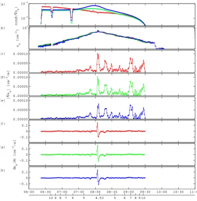
Fig. 6. Computation of∇xtne with isotropic homogeneity domain (red), anisotropic domain (green), and

anisotropic domain with small-scale fluctuations (blue) (see text). (a) condition number; (b)neobserved by the

four spacecraft; (c–e) magnitude of spatial gradient|∇ne|; (f–h) temporal gradient∂ne/∂t. The bottom scale

gives theL-shell position of the center of the Cluster tetrahedron.

28

Fig. 6. Computation of∇_xtnewith isotropic homogeneity domain (red), anisotropic domain (green), and anisotropic domain with small-scale fluctuations (blue) (see text). (a) condition number; (b)neobserved by the four spacecraft; (c–e) magnitude of spatial gradient|∇ne|; (f–h) temporal gradient∂ne/∂t. The bottom scale gives theL-shell position of the center of the Cluster tetrahedron.

is a double-peaked spatial gradient around 08:05 UT corre-sponding to the rising and falling slopes around the density peak observed near perigee (compare with panel b). There are also important gradients (∼0.05 cm−3/km, relative pre-cision 10%) near 07:50 UT and near 08:15 UT. These strong gradients are identical to those reported by Darrouzet et al. (2006b) and interpreted there as proof of azimuthal structure. As the densities drop farther away from Earth, the gradients tend to become negligible well before and after perigee. The temporal gradient is pretty small (<0.01 cm−3/s with a rela-tive precision of 20% at best), except for the bipolar structure near perigee, which corresponds to the convection of the den-sity structure. The three results are almost identical, but the error margins are again smallest (<8%) for the case of an anisotropic homogeneity domain.

Comparing∇_xtnefor the anisotropic case to the instanta-neous spatial gradients without or with fluctuations (Fig. 7), the two instantaneous spatial gradients are necessarily found to be equal and there are only minor differences with the space-time gradient (panel c, d, and e). The condition num-ber is not much different between the three computations (panel a), but it clearly is best for the space-time gradient. The space-time gradient also has the smallest error margins.

7 Gradients of a vector field

J. De Keyser et al.: Least-squares gradient calculation 981

(f)

10 9 8 7 6 5 4.53 5 6 7 8 9 10 (e)

06:00 06:30 07:00 07:30 08:00 08:30 09:00 09:30 10:00 10:30 11:00 0.00000

0.00005 0.00010 (d)

|

∇

ne

| [cm

−3

/m]

0.00000 0.00005 0.00010 (c)

0.00000 0.00005 0.00010 (b)

ne

[cm

−3

] 10 2

(a)

cond(

∇

ne

)

10−4 10−2

Fig. 7. Computation of∇newith anisotropic homogeneity domain and fluctuations (red), with the

instanta-neous gradient version (green), and with the instantainstanta-neous version with fluctuations (blue) (see text). (a)

con-dition number; (b)neobserved by the four spacecraft; (c–e) magnitude of spatial gradient|∇ne|. The bottom

scale gives theL-shell position of the center of the Cluster tetrahedron.

29

Fig. 7. Computation of∇newith anisotropic homogeneity domain and fluctuations (red), with the instantaneous gradient version (green), and with the instantaneous version with fluctuations (blue) (see text). (a) condition number; (b)neobserved by the four spacecraft; (c– e) magnitude of spatial gradient|∇ne|. The bottom scale gives theL-shell position of the center of the Cluster tetrahedron.

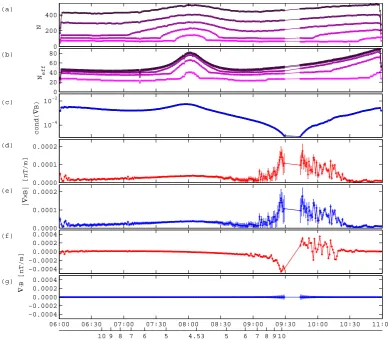
components independently or coupling them through the zero-divergence constraint. From them,∇×Band∇·Bare ob-tained, as shown in Fig. 8. The effective scale factor is close to unity (as for the∇_xt|B|computation in Sect. 6).Seff,N, andNeffare identical for both computations. The number of equationsN (panel a) is three times larger than for a scalar field. BothNandNeff(panel b) peak near perigee as a con-sequence of the alignment between the spacecraft orbits and the direction with the longest homogeneity scale length (the magnetic field direction). The condition number is identical for both computations (panel c), although the overdetermined system sizes are different (same data used, but only 14 un-knowns in the divergence-free case, rather than 15). The pro-gressively deteriorating condition number toward 09:40 UT reflects the spacecraft coplanarity issue. The condition num-ber is quite good elsewhere. The curl (panels d and e) and the divergence (panels f and g) from the uncoupled and the divergence-free computations have absolute error margins of typically 0.005 nT/km (a relative error of 10% on|∇×B|). Away from the coplanarity time interval,∇·B does not sig-nificantly deviate from zero. The correction of the solution implied by requiring∇·B=0 is rather small. While the least-squares method minimizes the differences between the ob-servations and the linear approximation, adding a constraint limits the solution search space so that the error margins be-come slightly larger. Nevertheless, adding physically rele-vant constraints obviously improves the realism of the solu-tion.

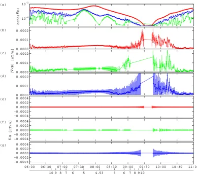
Figure 9 compares the curl (panels b, c, and d) and di-vergence (panels e, f, and g) for the didi-vergence-free spatio-temporal gradient computation as well as for the divergence-free instantaneous gradient computation, applied to 60 s av-eraged data, without and with small-scale fluctuations, re-spectively. While the results of the computations are essen-tially the same, the condition number (panel a) is best for the spatio-temporal gradient. It occasionally drops below 10−5 for the instantaneous gradient without fluctuations. The error margins are smallest for the spatio-temporal gradient despite the fact that only the spatio-temporal gradient error estimates account for the three error sources (measurement error, cur-vature error, and fluctuation error).

8 Physical relevance

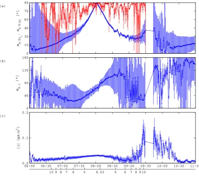
In order to illustrate the usefulness of these gradients for scientific analysis, Fig. 10a shows the angles αB,∇|B| and αB,∇ne between the ambient magnetic field B on the one

(g)

06:00 06:30 07:00 07:30 08:00 08:30 09:00 09:30 10:00 10:30 11:00 −0.0004

−0.0002 0.0000 0.0002 0.0004 (f)

∇

⋅

B [nT/m]

−0.0004 −0.0002 0.0000 0.0002 0.0004 (e)

0.0000 0.0001 0.0002 (d)

|

∇

×

B| [nT/m]

0.0000 0.0001 0.0002 (c)

cond(

∇

B)

10−4 10−2 (b)

Neff

0 20 40 60 80

10 9 8 7 6 5 4.53 5 6 7 8 9 10 (a)

N

0 200 400

Fig. 8. Computation of∇×Band∇·Bevery60 swith anisotropic homogeneity domain and fluctuations (see

text) without (red) and with (blue) the∇·B= 0constraint. (a) number of equationsNin the overdetermined

system, with each curve referring to a thresholdσk; (b) effective number of equationsNeff; (c) problem

condi-tion number; (d–e) magnitude of the curl|∇×B|, with growing error bars and gap in the computed gradient

due to spacecraft coplanarity; (f–g) divergence∇·B. The bottom scale gives theL-shell position of the center

of the Cluster tetrahedron.

30

Fig. 8. Computation of∇×Band ∇·B every 60 s with anisotropic homogeneity domain and fluctuations (see text) without (red) and with (blue) the∇·B=0 constraint. (a) number of equationsNin the overdetermined system, with each curve referring to a thresholdσk; (b) effective number of equationsNeff; (c) problem condition number; (d–e) magnitude of the curl|∇×B|, with growing error bars and gap in the computed gradient due to spacecraft coplanarity; (f–g) divergence∇·B. The bottom scale gives theL-shell position of the center of the Cluster tetrahedron.

2006a,b). As we are only interested in the direction of these gradients, not their sense, the angles are reduced to the in-terval[0◦,90◦]. By definition, the magnetic field strength gradient is perpendicular toBat the magnetic equator, cor-responding to αB,∇|B|=90◦, near 08:02 UT (close to, but not exactly at Cluster perigee). Before and after that time, as the Cluster spacecraft are at higher magnetic latitudes, that angle decreases rapidly because of the progressively more important field-aligned gradient. The error margins are large away from perigee as bothB and∇|B| are small there. AngleαB,∇ne remains quite large throughout the time

interval, indicating that∇||ne∇⊥ne at the relatively low latitudes Cluster is sampling, something that has also been found with radio sounding techniques (Reinisch et al., 2001). This is due to a small longitudinal gradient within each flux tube, but also because of the existence of strong radial and azimuthal density structure on the transverse homogeneity scale of 500 km adopted here. The gradient orientations

ob-tained here compare very well to the instantaneous gradient directions reported by Darrouzet et al. (2006b).

Assuming that there are no time changes in the electric field, the current densityj=∇×B/µ0can be readily com-puted from the curl of the magnetic field. The angleαB,j

betweenB andj as well as the current density magnitude

|j|are given in Figs. 10b and c (anisotropic divergence-free vector case with fluctuations). The current density vectorj

is perpendicular toB somewhat northward of the magnetic equator, around 08:10 UT. Close to perigee,αB,j is<90◦

J. De Keyser et al.: Least-squares gradient calculation 983

(g)

06:00 06:30 07:00 07:30 08:00 08:30 09:00 09:30 10:00 10:30 11:00 −0.0004

−0.0002 0.0000 0.0002 0.0004 (f)

∇

⋅

B [nT/m]

−0.0004 −0.0002 0.0000 0.0002 0.0004 (e)

−0.0004 −0.0002 0.0000 0.0002 0.0004 (d)

0.0000 0.0001 0.0002 (c)

|

∇

×

B| [nT/m]

0.0000 0.0001 0.0002 (b)

0.0000 0.0001 0.0002

10 9 8 7 6 5 4.53 5 6 7 8 9 10 (a)

cond(

∇

B)

10−4 10−2

Fig. 9. Computation of∇×Band∇·B, subject to the∇·B= 0constraint, with anisotropic homogeneity domain

and fluctuations (red), with the instantaneous gradient version (green), and with the instantaneous version with

fluctuations (blue) (see text). (a) condition number; (b–d) magnitude of the curl|∇×B|; (f–g) divergence∇·B.

The bottom scale gives theL-shell position of the center of the Cluster tetrahedron.

31

Fig. 9. Computation of∇×Band∇·B, subject to the∇·B= 0 constraint, with anisotropic homogeneity domain and fluctuations (red), with the instantaneous gradient version (green), and with the instantaneous version with fluctuations (blue) (see text). (a) condition number; (b–d) magnitude of the curl|∇×B|; (f–g) divergence∇·B. The bottom scale gives theL-shell position of the center of the Cluster tetrahedron.

9 Conclusions

This paper describes a general-purpose method for comput-ing gradients of scalar and vector fields in space and time. It has been shown that (1) The weighted least-squares method for computing gradients is a very robust one. (2) The method provides reliable error estimates that include the effects of measurement errors and approximation errors due to struc-ture at scales that are larger and/or smaller than the physical scale of interest. (3) The method provides diagnostics to as-sess the quality of the computation, in particular by monitor-ing the smonitor-ingular values of the problem as a generalization of the concepts of planarity or elongation of a 4-spacecraft con-figuration. The role of the different parameters of the gradi-ent computation algorithm has been illustrated. The relative importance of the different types of errors and their effect on the quality of the results has been discussed.

The method has been found to be superior to the traditional instantaneous gradient computation. Its primary advantage is

its generality and its robustness. It correctly applies the prin-ciple of locality of information since only local data are used to compute the gradient at any given point, in accordance with the homogeneity condition. It also yields more strin-gent error margins on the obtained gradients. A disadvantage is its mathematical complexity. Implementing the method is not trivial. Computing the gradients is time-consuming when one considers small-scale fluctuations (f∗6=0), because then the (possibly large) error covariance matrices must be diago-nalized. While the gradients obtained with this new method typically do not differ very much from those obtained with the traditional instantaneous gradient method, one now ob-tains a quantitative estimate of the total error on the results.

(c)

|j| [

µ

A/m

2]

06:00 06:30 07:00 07:30 08:00 08:30 09:00 09:30 10:00 10:30 11:00 0.0

0.1 0.2 (b)

αB,j

[°]

0 45 90 135 180

10 9 8 7 6 5 4.53 5 6 7 8 9 10 (a)

αB,

∇

ne

,

αB,

∇

|B|

[°]

0 15 30 45 60 75 90

Fig. 10. Orientation of gradients during the Cluster inner magnetosphere pass on August 7, 2003, as a

func-tion of time and ofL-shell. (a) AngleαB,∇|B| (blue) andαB,∇ne (red) betweenB and∇|B|and∇ne,

respectively (anisotropic homogeneity with fluctuations, see text), reduced to[0◦,90◦]. The magnetic

equa-tor corresponds toαB,∇|B| = 90◦, near 08:02 UT. Both angles reflect the relative proportion of parallel and

perpendicular gradients;∇|||B|is rather strong away from the equator, while∇||ne ∇⊥nedue to small

longitudinal gradients within each flux tube and because of radial and azimuthal density structure. (b) Angle

αB,jbetweenBand current densityj(wherej =∇×B/µ0in a steady situation). (c) Current density

mag-nitude|j|is significantly different from zero in the plasmasphere, indicating deviation from a dipolar field. The

current density vector contains a significant field-aligned component inside the plasmasphere (around perigee)

and also on auroral field lines (just after 06 UT).

32

Fig. 10. Orientation of gradients during the Cluster inner magnetosphere pass on 7 August 2003, as a function of time and ofL-shell. (a) AngleαB,∇|B| (blue) andαB,∇ne (red) betweenB and∇|B|and∇ne, respectively (anisotropic homogeneity with fluctuations, see

text), reduced to[0◦,90◦]. The magnetic equator corresponds toαB,∇|B|=90◦, near 08:02 UT. Both angles reflect the relative proportion of parallel and perpendicular gradients;∇|||B|is rather strong away from the equator, while∇||ne∇⊥nedue to small longitudinal gradients within each flux tube and because of radial and azimuthal density structure. (b) AngleαB,j betweenBand current density j (where

j=∇×B/µ0in a steady situation). (c) Current density magnitude|j|is significantly different from zero in the plasmasphere, indicating deviation from a dipolar field. The current density vector contains a significant field-aligned component inside the plasmasphere (around perigee) and also on auroral field lines (just after 06:00 UT).

however, is always possible. Once the gradient is computed along the spacecraft trajectory, one can check how it changes with position and/or with time, at least to a certain extent, so that an evaluation can be made of the curvature error. As long as there are enough points within the homogeneity domain, the value and the precision of the gradient are determined mainly by the measurement and fluctuation errors, and the exact value of the curvature error is not too important. A limitation of the present method is that a single, fixed value for the curvature error parameterfc is used throughout the domain. Another limitation is that we have not accounted for timing errors or spacecraft position errors.

As an illustration, this method was used to analyze mag-netic field and plasma density data obtained by Cluster dur-ing a pass through the inner magnetosphere. The relative importance of the perpendicular and field-aligned gradients

of the magnetic field strength and of the plasma density have been discussed. In addition, nonzero current densities have been found, indicating that the field is not dipolar. Field-aligned currents appear to exist in the outer regions of the plasmasphere and on auroral field lines. The correct eval-uation of the error margins on the gradients offered by the proposed method is absolutely necessary to ascertain the re-liability of these findings.

J. De Keyser et al.: Least-squares gradient calculation 985 method will always produce a result, but whether the

com-puted gradients are accurate depends on the nature of the data. With Cluster, a good gradient can usually be obtained when the homogeneity scales are on the order of, or larger than, the spacecraft separations in space and time.

Appendix A

Constraints

The overdetermined system (2) may still be ill-conditioned as the redundancy that stems from repeatedly measuring the same quantity over time on different spacecraft may be rather limited. For example, if the spacecraft are all in the same orbital plane, it is impossible to extract information about variations in the direction perpendicular to that plane. This ill-conditioning can be avoided if one adds new information about the problem in the form of constraints.

We discuss here two types of (linear) constraints that may be very useful in practice: geometrical ones, which state that one or more spatial gradient components are zero, and the stationarity constraint, which specifies that the total time derivative is zero.

A1 Geometrical constraints

Geometrical constraints are introduced by specifying an or-thonormal set of vectors cj, j=1, . . . , m (m≤3) to which ∇_xtf0 must be perpendicular. For example, the gradient might be required to be perpendicular to the local mag-netic field vector B. In that case, m=1 and c1=B/kBk. A set of orthonormal vectors di, i=1, . . . ,4−mcan then be constructed, so that di>cj=0. Transforming any vec-tor asxβ=[. . .di. . .cj. . .]>x, the gradient itself becomes [. . .di. . .cj. . .]>∇xtf0. Since cj>∇xtf0=0, the m last components of the gradient vanish. The directions cj can thus be regarded as homogeneity directions correspond-ing to infinite homogeneity scales, since the gradient must be invariant (identically zero) in each of those directions, so thatU=[. . .dj. . .cj. . .]andL=diag([. . . lj. . .+ ∞...]). TransformationPis now a projection rather than a rotation and scaling (the space spanned by thecj is its null space), its target space being (4−m)-dimensional. The constraint generally improves problem conditioning, but leads to larger residuals as there is less freedom to mimimizer>r.

As an example, consider the situation in which the gra-dient direction in space is known, say, that it lies alongx. Thenc1=[0;1;0;0]andc2=[0;0;1;0]. For time-separable homogeneity with length scalelx=ly=lz=ξ and time scale lt=τ, one finds

U=



  

1 0 0 0

0 0 1 0

0 0 0 1

0 1 0 0



  

andL= 

  

ξ 0 0 0

0 τ 0 0

0 0 +∞ 0

0 0 0 +∞



   ,

which leads to a projectionxβ=x/ξ,tβ=t /τ. A2 Stationarity constraint

For a structure moving with a given constant velocity v0, time-stationarity is expressed by

df0

dt = [v0 1] >

∇xtf0=0.

This constraint corresponds to an infinite homogeneity scale along directionu4∝[ v0 1]. Homogeneity in time is not separable from homogeneity in space unlessv0=0.

As an example, considerv0=[v0;0;0]. Homogeneity di-rections u1, u2, andu3 must form an orthonormal set to-gether withu4. One particular choice produces

U=       1/ q

v₀2+1 0 0 v0/ q

v2₀+1

0 1 0 0

0 0 1 0

−v0/ q

v₀2+1 0 0 1/ q

v2₀+1       and L=      ξ / q

v₀2+1 0 0 0

0 ξ 0 0

0 0 ξ 0

0 0 0 +∞

     ,

whereξ is a length scale. The projection turns out to be xβ=(x−v0t )/ξ,yβ=y/ξ,zβ=z/ξ, so that one actually com-putes the spatial gradient with isotropic homogeneity length scalelx=ly=lz=ξ in a reference frame that moves withv0.

Appendix B

Cross-correlations of small-scale perturbations

We restrict ourselves to distributions of small-scale perturba-tions that are isotropic inγ-space with perturbation strength dropping off exponentially. The mean perturbation ampli-tude is assumed constant over the homogeneity domain, such that

h(δfssλ(λ,x))2i =δfλ2(λγ)=16f∗2S4( 4 Y k=1 ˆ λk)e −λγ

(λγ₎3,

with λγ=kλk_γ, f∗ a constant, and S4 the surface of a 4-dimensional sphere. Because of the locality of the perturbations,hδfssλ(λ,xi)δfssλ(λ,xj)i≈δfλ2(λγ)when 1x_ijγ=kxj−xikγλγ and zero when1xijγλγ. For sim-plicity, the switch between both situations is taken to be an abrupt one. The covariances ofδfssat pointsx_i andx_j can then be computed as

hδfss(xi)δfss(xj)i (B1) =

Z

λ

Z

λ0

= Z

λ

hδfssλ(λ,xi)δfssλ(λ,xj)idλ

≈( 4 Y

k=1 ˆ λk)

S4 16

Z +∞

1x_ijγ

(λγ)3δf_λ2(λγ)dλγ (B2)

=f∗2e−1x

γ

ij_{, (B3)}

wheref∗2is the total perturbation variance. Whatever the specific choice of perturbation amplitude distribution, it must decrease faster than 1/(λγ)3in order to obtain a finite total perturbation, and the end result will always be that the cross-correlation is large between nearby points, and becomes zero as the distance between both points exceeds the perturbation length scale.

Acknowledgements. The authors thank M. Hamrin for fruitful

dis-cussions. This work was supported by the Belgian Federal Of-fice for Scientific, Technical and Cultural Affairs through ESA (PRODEX/Cluster and PRODEX/Solar Drivers of Space Weather). Topical Editor I. A. Daglis thanks M. L. Adrian and C. Harvey for their help in evaluating this paper.

References

Balogh, A., Dunlop, M. W., Cowley, S. W. H., Southwood, D. J., Thomlinson, J. G., Glassmeier, K.-H., Musmann, G., L¨uhr, H., Buchert, S., Acu˜na, M. H., Fairfield, D. H., Slavin, J. A., Riedler, W., Schwingenschuh, K., Kivelson, M. G., and the Cluster mag-netometer team: The Cluster Magnetic Field Investigation, Space Sci. Rev., 79, 65–91, 1997.

Balogh, A., Carr, C. M., Acu˜na, M. H., Dunlop, M. W., Beek, T. J., Brown, P., Fornac¸on, K.-H., Georgescu, E., Glassmeier, K.-H., Harris, J., Musmann, G., Oddy, T., and Schwingenschuh, K.: The Cluster Magnetic Field Investigation: overview of in-flight performance and initial results, Ann. Geophys., 19, 1207–1217, 2001,

http://www.ann-geophys.net/19/1207/2001/.

Carpenter, D. L. and Lemaire, J.: Erosion and recovery of the plas-masphere in the plasmapause region, Space Sci. Rev., 80, 153– 179, 1997.

Carpenter, D. L. and Lemaire, J.: The Plasmasphere Boundary Layer, Ann. Geophys., 22, 4291–4298, 2004,

http://www.ann-geophys.net/22/4291/2004/.

Chanteur, G.: Spatial Interpolation for Four Spacecraft: The-ory, in: Analysis Methods for Multi-Spacecraft Data, edited by Paschmann, G. and Daly, P. W., pp. 349–369, ISSI Scientific Re-port SR-001, 1998.

Chanteur, G. and Harvey, C. C.: Spatial Interpolation for Four Spacecraft: Application to Magnetic Gradients, in: Analysis Methods for Multi-Spacecraft Data, edited by: Paschmann, G. and Daly, P. W., pp. 371–393, ISSI Scientific Report SR-001, 1998.

Darrouzet, F., D´ecr´eau, P. M. E., De Keyser, J., Masson, A., Gal-lagher, D. L., Santolik, O., Sandel, B. R., Trotignon, J. G., Rauch, J. L., Le Guirriec, E., Canu, P., Sedgemore, F., Andr´e, M., and Lemaire, J. F.: Density structures inside the plasmasphere: Clus-ter observations, Ann. Geophys., 22, 2577–2585, 2004, http://www.ann-geophys.net/22/2577/2004/.

Darrouzet, F., De Keyser, J., D´ecr´eau, P. M. E., Gallagher, D. L., Pierrard, V., Lemaire, J. F., Sandel, B. R., Dandouras, I., Matsui, H., Dunlop, M. W., Cabrera, J., Masson, A., Canu, P., Trotignon, J.-G., Rauch, J.-L., and Andr´e, M.: Analysis of plasmaspheric plumes: CLUSTER and IMAGE observations, Ann. Geophys., 24, 1737–1758, 2006a.

Darrouzet, F., De Keyser, J., D´ecr´eau, P. M. E., Lemaire, J. F., and Dunlop, M. W.: Spatial gradients in the plas-masphere from Cluster, Geophys. Res. Lett., 33, L08 105, doi:10.1029/2006GL025727, 2006b.

D´ecr´eau, P. M. E., Fergeau, P., Krasnoselskikh, V., L´evˆeque, M., Martin, P., Randriamboarison, O., Sen´e, F. X., Trotignon, J. G., Canu, P., M¨ogensen, P. B., and Whisper investigators: WHIS-PER, A Resonance Sounder and Wave Analyser: Performances and Perspectives for the Cluster Mission, Space Sci. Rev., 79, 157–193, 1997.

D´ecr´eau, P. M. E., Fergeau, P., Krasnoselskikh, V., Le Guirriec, E., L´evˆeque, M., Martin, P., Randriamboarison, O., Rauch, J. L., Sen´e, F. X., S´eran, H. C., Trotignon, J. G., Canu, P., Cornil-leau, N., de F´eraudy, H., Alleyne, H., Yearby, K., M¨ogensen, P. B., Gustafsson, G., Andr´e, M., Gurnett, D. A., Darrouzet, F., Lemaire, J., Harvey, C. C., Travnicek, P., and Whisper experi-menters: Early results from the Whisper instrument on Cluster: an overview, Ann. Geophys., 19, 1241–1258, 2001,

http://www.ann-geophys.net/19/1241/2001/.

D´ecr´eau, P. M. E., Le Guirriec, E., Rauch, J. L., Trotignon, J. G., Canu, P., Darrouzet, F., Lemaire, J., Masson, A., Sedgemore, F., and Andr´e, M.: Density irregularities in the plasmasphere bound-ary player: Cluster observations in the dusk sector, Adv. Space Res., 36, 1964–1969, 2005.

Dunlop, M. W. and Balogh, A.: Magnetopause current as seen by Cluster, Ann. Geophys., 23, 901–907, 2005,

http://www.ann-geophys.net/23/901/2005/.

Dunlop, M. W., Balogh, A., Glassmeier, K.-H., and Robert, P.: Four-point Cluster application of magnetic field analy-sis tools: The Curlometer, J. Geophys. Res., 107, 1384, doi:10.1029/2001JA0050088, 2001.

Dunlop, M. W., Balogh, A., Shi, Q.-Q., Pu, Z., Vallat, C., Robert, P., Haaland, S., Shen, C., Davies, J. A., Glassmeier, K.-H., Cargill, P., Darrouzet, F., and Roux, A.: The Curlometer and other gra-dient measurements with Cluster, Proceedings of the Cluster and Double Star Symposium, 5th Anniversary of Cluster in Space, ESA SP-598, 2006.

Harvey, C. C.: Spatial Gradients and the Volumetric Tensor, in: Analysis Methods for Multi-Spacecraft Data, edited by: Paschmann, G. and Daly, P. W., pp. 307–322, ISSI Scientific Re-port SR-001, 1998.

Lemaire, J. F. and Gringauz, K. I.: The Earth’s Plasmasphere, Cam-bridge University Press, CamCam-bridge, 1998.

Rauch, J. L., Suraud, X., D´ecr´eau, P. M. E., Trotignon, J. G., Led´ee, R., Lemercier, G., El-Lemdani Mazouz, F., Grimald, S., Bozan, G., Valli`eres, X., Canu, P., and Darrouzet, F.: Automatic determination of the plasma frequency using image processing on WHISPER data, Proceedings of the Cluster and Double Star Symposium, 5th Anniversary of Cluster in Space, ESA SP-598, 2006.

Ob-J. De Keyser et al.: Least-squares gradient calculation 987

servations From IMAGE, Geophys. Res. Lett., 28, 4521–4524, doi:10.1029/2001GL013684, 2001.

Robert, P., Dunlop, M. W., Roux, A., and Chanteur, G.: Accuracy of Current Density Determination, in: Analysis Methods for Multi-Spacecraft Data, edited by: Paschmann, G. and Daly, P. W., pp. 395–418, ISSI Scientific Report SR-001, 1998a.

Robert, P., Roux, A., Harvey, C. C., Dunlop, M. W., Daly, P. W., and Glassmeier, K.-H.: Tetrahedron Geometric Factors, in: Analysis Methods for Multi-Spacecraft Data, edited by: Paschmann, G. and Daly, P. W., pp. 323–348, ISSI Scientific Report SR-001, 1998b.

Trotignon, J. G., D´ecr´eau, P. M. E., Rauch, J. L., Randriamboari-son, O., Krasnoselskikh, V., Canu, P., Alleyne, H., Yearby, K., Le Guirriec, E., S´eran, H. C., Sen´e, F. X., Martin, P., L´evˆeque, M., and Fergeau, P.: How to determine the thermal electron density and the magnetic field strength from the CLUS-TER/WHISPER observations around the Earth, Ann. Geophys., 19, 1711–1720, 2001,

http://www.ann-geophys.net/19/1711/2001/.

Trotignon, J. G., D´ecr´eau, P. M. E., Rauch, J. L., Le Guirriec, E., Canu, P., and Darrouzet, F.: The Whisper Relaxation Sounder Onboard Cluster: A Powerful Tool for Space Plasma Diagnosis around the Earth, Cosmic Research, 41, 369–372, 2003. Trotignon, J. G., D´ecr´eau, P. M. E., Rauch, J. L., Suraud, X.,

Grimald, S., El-Lemdani Mazouz, F., Valli`eres, X., Canu, P., Darrouzet, F., and Masson, A.: The electron density around the Earth, a high level product of the CLUSTER/WHISPER relax-ation sounder, Proceedings of the Cluster and Double Star Sym-posium, 5th Anniversary of Cluster in Space, ESA SP-598, 2006. Vallat, C., Dandouras, I., Dunlop, M., Balogh, A., Lucek, E., Parks, G. K., Wilber, M., Roelof, E. C., Chanteur, G., and R`eme, H.: First current density measurements in the ring current region us-ing simultaneous multi-spacecraft CLUSTER-FGM data, Ann. Geophys., 23, 1849–1865, 2005,