www.ann-geophys.net/28/1723/2010/ doi:10.5194/angeo-28-1723-2010
© Author(s) 2010. CC Attribution 3.0 License.
Annales
Geophysicae
Observations and modelling of the wave mode evolution of an
impulse-driven 3 mHz ULF wave
J. D. Borderick1, T. K. Yeoman1, C. L. Waters2, and D. M. Wright1
1Dept. of Physics and Astronomy, University of Leicester, University Road, Leicester, LE1 7RH, UK
2School of Mathematical and Physical Sciences, The University of Newcastle, Callaghan, 2308, New South Wales, Australia Received: 14 May 2010 – Revised: 26 July 2010 – Accepted: 7 September 2010 – Published: 22 September 2010
Abstract. A combination of an HF Doppler sounder, a net-work of ground magnetometers, upstream solar wind moni-tors and a numerical model is used to examine the temporal evolution of an Ultra Low Frequency (ULF) wave. The event occurred on 16 April 1998 and followed a solar wind den-sity and pressure increase seen in the upstream ACE space-craft data. The magnetometer and HF Doppler sounder data show that the event develops into a low-m (−6) field line resonance. HF signals that propagate via the ionosphere ex-hibit Doppler shifts due to a number of processes that give rise to a time-dependent phase path. The ULF electric and magnetic fields are calculated by a one-dimensional model which calculates the wave propagation from the magneto-sphere, through the ionosphere to the ground with an oblique magnetic field. These values are then used to determine a model HF Doppler shift which is subsequently compared to HF Doppler observations. The ULF magnetic field at the ground and Doppler observations are then used to provide model inputs at various points throughout the event. We find evidence that the wave mode evolved from a mixture of fast and Alfvén modes at the beginning of the event to an almost purely shear Alfvénic mode after 6 wavecycles (33 min). Keywords. Ionosphere (Ionosphere-magnetosphere interac-tions; Wave propagation) – Magnetospheric physics (MHD waves and instabilities)
1 Introduction
ULF plasma waves in the 1–100 mHz range are ubiquitous in the Earth’s magnetosphere. These waves are an impor-tant coupling mechanism between the magnetosphere and
Correspondence to: J. D. Borderick
the ionosphere, since they transfer both momentum and en-ergy. The coupling processes are most significant in the high-latitude ionosphere, where the ULF wave amplitudes are the largest. The waves also act as an important diagnostic of magnetospheric dynamics and morphology.
When the frequency of the incoming wave matches the local resonant frequency of a geomagnetic field line then a Field Line Resonance (FLR) will occur (Chen and Hasegawa, 1974a; Southwood, 1974). In this process an in-coming compressional fast-mode wave couples to an Alfvén mode oscillation on a geomagnetic field line of a matching eigenfrequency. The source of the fast mode waves was as-sumed to be Kelvin-Helmholtz (K-H) driven surface waves on the magnetospheric flanks caused by solar wind flow (Kivelson and Pu, 1984). FLRs have large spatial scale in longitude, but develop small scale structures in the latitudi-nal direction.
This paper investigates an impulsively excited pulsation. Such phenomena have been studied over a considerable pe-riod both experimentally (e.g., Siebert, 1964; Matsushita and Saito, 1967; Voelker, 1968) and theoretically (Tamao, 1965; Chen and Hasegawa, 1974b). In the case of an impulsively excited wave the source of the compressional mode lies in the impulse, with this transient compressional mode then coupling to the Alfvén mode oscillation on a geomagnetic field line similarly to the more steady-state picture described above. More recent observational, theoretical and modelling studies (e.g., Kivelson et al., 1984; Allan et al., 1986,b; Kivelson and Southwood, 1986; Lee and Lysak, 1989; Sam-son, 1991) have subsequently developed the idea that follow-ing an impulse to, or solar wind buffetfollow-ing of, the magneto-sphere, it is the dimensions of the magnetospheric cavity that determine the eigenfrequencies of cavity or waveguide mode waves. These modes then couple to Alfvén modes, driving FLRs at discrete, harmonically related frequencies.
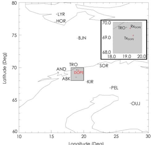
Fig. 1. The locations of the ground based instrumentation used
dur-ing this study. The red crosses represent the locations of the DOPE (Doppler Pulsation Experiment) sounder and the black crosses rep-resent the locations of the ten IMAGE magnetometer stations used in this study. The grey shaded square shows a zoomed in view of the DOPE site highlighting both the location of the transmitter (Tx) and Receiver (Rx) sites relative to the IMAGE magnetometer at Tromsø (TRO).
(e.g., Yeoman et al., 1990) and hence controls the transfer of momentum and energy. It is well known that MHD waves propagate through the magnetosphere, interact with the iono-sphere and may be detected on the ground using magnetome-ters. The ionosphere, atmosphere and ground introduce im-portant effects that alter the amplitude and polarisation of these waves leading to rotation and attenuation of the wave magnetic signatures detected on the ground (Hughes and Southwood, 1976b). Remote sensing of the magnetosphere is, therefore, only possible if the effects of the ionosphere and atmosphere are included. It is important therefore, to develop the theoretical models explaining the interaction of such atmospheric layers. The ionospheric signature of ULF waves is thus an important research area.
Oscillations in radio waves reflected from the ionosphere (Doppler frequency oscillations) are often correlated with os-cillations recorded by ground-based magnetometers (Davies et al., 1962). A theory to describe the relationship between these oscillations was proposed by Rishbeth and Garriott (1964). The theory explained that the Doppler frequency os-cillations were due to the ULF electric field, causing a verti-cal bulk motion of electrons in the ionosphere. The vertiverti-cal motion is the vertical component of theE∧Bplasma drift velocity. This is known as the advection mechanism. Poole
and Sutcliffe (1988) developed this idea explaining that there were in fact three mechanisms which can contribute to the observed Doppler shift. The first mechanism was the mag-netic mechanism. This mechanism results from the changes in refractive index due to changes in the ULF magnetic field intensity. Hence, this mechanism requires no bodily move-ment of electrons. The second mechanism was the advec-tion mechanism already identified by Rishbeth and Garriott (1964). The third mechanism was the compression mech-anism. This results from the changes in refractive index brought about due to changes in the local plasma density. This change is due to the redistribution of electrons caused by the compression and/or rarefaction induced by the ULF wave.
There have been a number of papers detailing aspects of the Doppler oscillations of vertically incident radio waves correlated with ULF geomagnetic pulsations (e.g., Poole and Sutcliffe, 1988; Wright et al., 1997). However, to fully match a theoretical model to reality, observational inputs are required. Ground based magnetometers and HF Doppler sounders can provide this input. HF Doppler sounders pro-vide measurements of the ionosphere at both a high spatial and temporal resolution and can probe different heights of the ionosphere by changing their sounding frequency. These sounders can thus provide important diagnostic information which can be used for comparison purposes with models of ULF wave activity.
This paper presents the first observations of a ULF wave mode evolving, from 09:45 UT to 10:45 UT, on 16 April 1998, from a mixture of fast and Alfvén modes at the be-ginning of the event to an almost purely shear Alfvénic mode after 6 wavecycles (33 min). The 1-D model of Sciffer et al. (2005) is used to model the wave observed by the HF Doppler sounder and ground based magnetometers.
2 Instrumentation 2.1 HF Doppler sounder
caused by changes in the phase path of the radio wave in the ionosphere (Bennett, 1967).
DOPE used a fixed-frequency, 4.45 MHz, continuous wave (CW) signal with a dual-channel receiver. The two channels discriminate between the O- and the X-mode sig-nals. These CW signals may be reflected from the ionosphere and mixed with a reference signal to calculate a frequency shift,1f, along the ray path (Wright et al., 1997). The fre-quency shift, in terms of the free space wavelength,λ, and the phase path of the signal,P, may be expressed as
1f= −1
λ dP
dt (1)
(Davies, 1962). If the change in phase path results purely from the motion of the reflection point in the ionosphere with a velocity,v, the frequency shift,1f, may be written as
1f= −2vf
c (2)
(Georges, 1967).
Sampling at the receiver, at 40 Hz, and processing through a Fast Fourier Transform (FFT) algorithm (512 points per FFT) provides a Doppler trace with a time resolution of 12.8 s. Here the Doppler trace is resampled from 12.8 s to 10.0 s. This resampling was conducted in order to make di-rect phase and amplitude comparisons between the data from DOPE and the IMAGE (International Monitor for Auroral Geomagnetic Effects) magnetometer instruments.
2.2 IMAGE magnetometer array
The ULF variations in the magnetic field were detected by the IMAGE network of triaxial fluxgate magnetometers (Luhr, 1994). The locations of the ten IMAGE magnetome-ters utilised during this study are presented in Fig. 1. The magnetometer data are sampled at 10 s intervals and are pre-sented in geographic coordinates.
2.3 Upstream interplanetary data
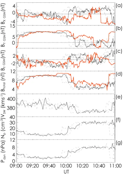
[image:3.595.310.547.60.395.2]Upstream solar wind and IMF conditions during the interval discussed in this paper were measured using the SWEPAM and MAG instruments, respectively, on the Advanced Com-position Explorer (ACE) spacecraft (Stone et al., 1998) and the IMP (Interplanetary Monitoring Platform)-8 spacecraft magnetometer (Armstrong et al., 1978). During the rele-vant interval on 16 April 1998, ACE was located in the solar wind near the Sun-Earth L1 Lagrangian point, at GSM co-ordinates (X, Y, Z) = (+233.69,−39.31,−4.52)RE. IMP-8 was located near the Earth-Sun line at GSM co-ordinates (X, Y, Z) = (+33.1,+6.4,+10.3)RE. During the period of inter-est the solar wind velocity was roughly 380 km s-1.
Fig. 2. ACE and IMP-8 spacecraft observations during the ULF wave event on 16 April 1998 between 09:00 UT–11:00 UT. netic field data are displayed in the GSM (Geocentric Solar Mag-netic) coordinate system. Panels (a) to (d) show the three magnetic field components recorded by the ACE and IMP-8 spacecraft, (Bx,
By,Bz) and the magnetic field magnitude,Btotal, respectively.
Pan-els (e), (f) and (g) show the solar wind velocity, the solar wind proton number density, and the solar wind dynamic pressure as recorded by ACE. The ACE data, with a 57 min lag are shown by the solid black lines, whereas the IMP-8 data, lagged by 14 min, are shown by the solid red lines. The dashed grey lines show a range of lag times (50–61 min) for the IMF and solar wind data as observed by ACE (see text for details).
3 Observations
3.1 IMF analysis
The origin of the ULF wave may be revealed by an ex-amination of upstream IMF and solar wind data. Figure 2 presents the lagged ACE and IMP-8 data sets for the ULF wave event on 16 April 1998 between 09:00 UT–11:00 UT. The ACE data, lagged by 57 min as predicted by the OMNI dataset (King and Papitashvili, 2005) are shown by the solid black lines and reveal a rise in dynamic pressure from 2 nPa to 7 nPa occurring at approximately 10:03 UT. This increase in dynamic pressure coincides with a rotation of the IMF, and a drop in magnetic field magnitude (and hence pressure). The plasma thermal pressure rises at this time (not shown), although the total pressure drops slightly. The IMF and solar wind data are thus consistent with the arrival of a tangen-tial discontinuity at this time. In order to confirm the va-lidity and accuracy of this applied lag, magnetic field data from the IMP-8 spacecraft are also examined (no plasma data are available from IMP-8). The solar wind propagation time from IMP-8 was found using the method of Khan and Cow-ley (1999). This technique for determining the lag time com-prises three parts: the solar wind advection time, the mag-netosheath transit time, and the Alfvén transit time along the geomagnetic field lines from the subsolar magnetopause to the ionosphere. The subsolar bow shock location is found using a model (Peredo et al., 1995). The transit time from the subsolar magnetopause to the ionosphere was approxi-mated as 2 min. The transit time from IMP-8 to the terrestrial ionosphere, using the solar wind velocity recorded by ACE as a guide, was determined to be 14.1±2 min. IMP-8 data at this lag are shown in Fig. 2 by the solid red lines. The IMP-8 data have been used to compare structures within the IMF at IMP-8 with those recorded by the ACE spacecraft. Cross-correlating the ACE data with the IMP-8 data for the total magnetic field and for each component of the IMF over a variety of timeseries lengths centred between 09:00 UT and 11:00 UT provided a range of time delays for the ACE data between 50 min and 61 min. The limits of these calculated lags on the ACE upstream data are presented in Fig. 2 as dashed grey lines, and indicate that the effect of the increase in solar wind dynamic pressure is expected to arrive in the ionosphere between 09:56 UT and 10:07 UT. This time inter-val is marked as a grey box on the time series of the ground-based measurements of the wave activity under investigation presented in Fig. 3. The interval is consistent with the ar-rival of the effects of the solar wind impulse being coinci-dent with the start of the wave event recorded in the ground magnetometer data, indicative of a wave source originating from the solar wind dynamic pressure impulse. An alterna-tive source of wave power on the ground is direct driving by oscillatory activity at a suitable frequency within the IMF or solar wind. An FFT analysis of the lagged ACE IMF and so-lar wind data reveals that between 09:45 UT–10:45 UT (and over the longer interval 07:00 UT–12:00 UT) the peak spec-tral power occurs at a frequency of approximately 2.0 mHz.
There is a little spectral power close to 3 mHz (the domi-nant frequency of the ground-based magnetometer data) at a steady level from 09:20 UT–11:00 UT in the lagged solar wind data which might result in weak steady state driving at 3 mHz, but the main wave source is consistent with the pres-sure impulse.
3.2 Ionospheric and ground observations
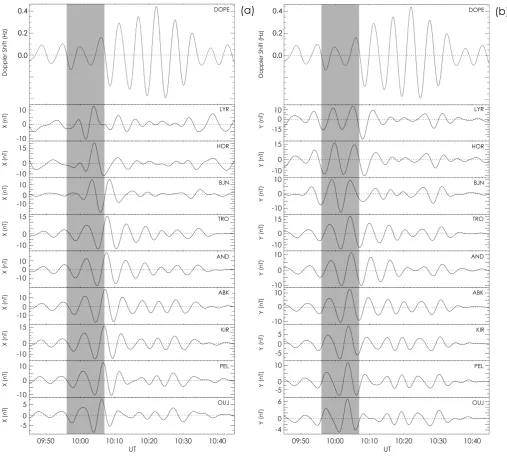
The top panels in Fig. 3 display HF Doppler data from DOPE, bandpass filtered between 250 s to 500 s (2 mHz– 4 mHz), along with identically filtered X and Y compo-nent magnetic field data from nine IMAGE magnetome-ter stations, covering geomagnetic latitudes from 75.12◦ (Longyearbyen, LYR), to 60.99◦(Oulujarvi, OUJ). The IM-AGE data are presented with latitude decreasing from top to bottom. A series of wave cycles are clearly visible in the data, which started at 09:45 UT and continued until about 10:45 UT. A coherent wave packet can be seen across the magnetometer chain, with maximum amplitude of 15 nT, at 10:08 UT, observed in the X component magnetic field be-tween the latitudes of TRO, and Abisko, (ABK). The wave signature in the magnetometer data was strongest in the in-terval 09:55 UT–10:30 UT.
The time development of the amplitudes in the Doppler and magnetometer traces is different, with peak amplitude seen early on in the wave packet in the magnetometer data (10:04 UT), but later in the Doppler trace (10:22 UT).
The grey shaded region on both panels of Fig. 3 shows the possible range of arrival times of the effects of the solar wind dynamic pressure increase as measured by the ACE space-craft, as determined in Fig. 2.
Fourier power spectral analysis of the DOPE instrument and the X and Y components of the data from the IMAGE magnetometer array reveal a consistent wave period of 330 s (3 mHz).
Fig. 3. DOPE and IMAGE Magnetometer data for the ULF wave event on 16 April 1998. Panels (a) and (b) display data from the X and
Y components of nine stations of the IMAGE magnetometer array bandpass filtered between 250 and 500 s. The upper panel in both (a) and (b) show the bandpass filtered DOPE data also excluding variations with time periods outside of the range 250 s to 500 s, resampled from 12.8 s to 10.0 s. The grey shaded region shows the possible range of arrival times of the effects of the solar wind dynamic pressure increase as measured by the ACE spacecraft. The time series plots have been scaled individually to provide the highest clarity of the wave signature.
3.3 Wave evolution
As mentioned in Sect. 3.2, the different temporal develop-ment observed in the amplitudes of the combined Doppler sounder and magnetometer datasets indicate an evolution in the wave mode, azimuthal or meridional scale-size of the wave. This evolution is investigated further here, through a dynamic Fourier analysis of the wave phase and
Fig. 4. IMAGE Magnetometer data for the ULF wave event on 16
April 1998. Panels (a) and (b) show the latitudinal Fourier power and phase profiles for the X component of the magnetic field, re-spectively. In both panels the overlaid dot-dash line shows the loca-tion of the DOPE instrument.
a frequency range of 1.7–5.1 mHz. The HF Doppler ampli-tude rises from 0.1 Hz at approximately 10:00 UT to a peak of 0.4 Hz at roughly 10:20 UT. Panels (b) and (c) show the TRO-X and TRO-Y amplitudes found using the same tech-nique as panel (a). Panel (b) shows TRO-X peaks with an amplitude of 15.0 nT at roughly 10:10 UT while panel (c) shows TRO-Y attaining a peak amplitude of 16.0 nT at ap-proximately 10:05 UT. Panel (d) of Fig. 5 shows the cross phase between the X component of IMAGE stations TRO and Pello (PEL), at the peak frequency of 3 mHz.
This cross phase calculation allows an examination of the time evolution of the relative phase between the wave signa-tures measured at the two stations. At the beginning of the wave event PEL leads TRO by approximately 60◦. As the wave progresses, this phase lead increases, maximising at ap-proximately 140◦between 10:15 UT and 10:25 UT. After this time the wave amplitudes start to decrease. The phase differ-ence between the stations thus starts with a small phase lead at the lower latitude station, evolving towards the 180◦phase lead expected between stations equatorward of and poleward of a field line resonance. This suggests a wave with an im-pulsive origin, which then exhibits a time dependent phase evolution as an FLR develops.
[image:6.595.307.548.63.380.2]Panel (e) of Fig. 5 shows a comparable analysis of the Y component of the magnetic field data from two azimuthally
Fig. 5. Panel (a) presents the HF Doppler amplitude variation
cal-culated from an integrated Fourier amplitude over a frequency range of between 1.7 mHz–5.1 mHz using a slip of 5 min. Panels (b) and
(c) show the TRO-X and TRO-Y amplitudes found using the same
technique as for panel (a). Panel (d) shows the X component cross phase between IMAGE stations TRO and PEL. Panel (e) shows the Y component cross phase between the azimuthally separated IM-AGE stations TRO and SOR. Panel (f) shows thekxtime evolution
determined from the ratio of the amplitudes of TRO-X and TRO-Y. The overplotted horizontal red dotted line shows the constant value ofkxassumed during the study. Panel (g) shows the implied ULF
wave mix evolution. The overplotted dot-dash lines show the 5 min intervals when the wave mix is calculated. The grey shaded region shows the possible range of arrival times of the effects of the solar wind dynamic pressure increase as measured by the ACE space-craft.
4 The numerical model 4.1 Introduction
The 1-D numerical model used here is that described in Scif-fer et al. (2005) which develops the existing work of Hughes (1974); Hughes and Southwood (1976b) and Zhang and Cole (1995). The new 1-D model formulates the altitude varia-tion of the ULF wave electric and magnetic fields, allows for an oblique geomagnetic background field,B0, and includes both Alfvénic and fast mode waves incident from the mag-netosphere.
As described in Waters et al. (2007), the ULF wave energy, which is incident from the magnetosphere, is described as an electromagnetic disturbance. The two required Maxwell equations are
∇∧E= −∂B
∂t (3)
and
∇∧H=J+∂D
∂t , (4)
where the current density,J, and the magnetic flux density, Bmay be expressed as
J=⇒σ E (5)
and
B=µH, (6)
where⇒σ is the conductivity tensor. The same Cartersian co-ordinate system as described in Sciffer and Waters (2002) is used here, where X is northward, Y is westward and Z is radially outward from the surface of the Earth. B0 lies in the XZ plane at an angleI to the horizontal. If there is no background electric field (E0=0) thenBandEmay be ex-pressed as
B=(B0cos(I ),0,B0sin(I ))+(bx,by,bz), (7)
and
E=(ex,ey,ez). (8)
If the ionospheric medium varies only in the vertical direc-tion, then the horizontal spatial and temporal dependence is
expi(kxx+kyy−ωt ) (9)
and the governing equations in their full component form may be written as
i "
ky2
ω − ω c2
ε11−
ε13ε31 ε33 # ex −i k
xky
ω + ω c2
ε12−ε13ε32
ε33
ey−iky
ε13 ε33
bx
+∂by
∂z +i kxε13
ε33
by=0, (10)
i k
xky
ω + ω c2
ε21−
ε23ε31 ε33 ex −i "
kx2 ω −
ω c2
ε22−ε23ε32
ε33 #
ey+iky
ε23 ε33
bx
+∂bx
∂z −i kxε23
ε33
by=0, (11)
iky
ε31 ε33ex+
∂ey
∂z +iky ε32
ε33ey+i ω− c2ky2
ωε33 !
bx
+ikxky
c2
ωε33by=0, (12) and
∂ex
∂z +ikx ε31 ε33
ex+ikx
ε32 ε33
ey−ikxky
c2 ωε33
bx
−i ω−c
2k2
x
ωε33 !
by=0, (13)
whereεij are the elements of the dielectric tensor, ε
(Wa-ters, 2006). The conductivity tensor,⇒σ, may be expressed in terms of the dielectric tensor,⇒ε, as
⇒
ε=⇒I − i
ε0ω
⇒
σ, (14)
where
⇒
I is the identity tensor (Zhang and Cole, 1995). Equa-tions (10), (11), (12) and (13) are four first order differential equations that only consider derivatives in the vertical direc-tion,Z. To complete the set, theez andbzULF wave field
components are
ez= −
ε31
ε33ex− ε32
ε33ey−ky c2
ωε33bx+kx c2
ωε33by (15) and
bz= −
ky
ωex+ kx
ωey. (16)
A total of four boundary conditions are required to solve the system. The ground specifies two of these. The Earth is as-sumed to be a uniform, homogenous conductor of finite con-ductivity. The ULF waves decay in amplitude in the medium due to the small frequency and are described by
∂ex
∂z −γ (σg,kx,ky,ω)ex=0 (17) and
∂ey
Fig. 6. Plasma frequency as a function of altitude for the ULF wave event at 10:04 UT on 16 April 1998. The green dots represent the O-mode ionogram trace and the red dots represent the X-Mode. The curved black line presents the dual Chapman function fitting to the POLAN inversion which is in blue. The red vertical line on the panel shows the DOPE transmission frequency. The reflection altitude for this event was 184 km. The vertical purple line shows the approximate frequency corresponding to peak FoF2.
The top boundary is set at 1000 km where resistive MHD plasma conditions are assumed. The model allows for the existence of both the shear Alfvén and fast mode waves up to the top boundary. For more information on the mathematical foundation of the numerical model see Sciffer et al. (2005).
In the model the atmospheric composition is found from a thermosphere model based on satellite mass spectrometer and ground-based incoherent scatter data (MSISE90) (Hedin et al., 1991). The ionospheric composition is found from the IRI model with the exception of the electron density pro-file, which is determined using the POLynomial ANalysis (POLAN) algorithm (Titheridge, 1985) and will be detailed in Sect. 4.2. The final step in the process is to calculate the Doppler shift contributions for the three mechanisms out-lined in the model of Poole and Sutcliffe (1988) and the Altar-Appleton-Hartree equation is used for this purpose. 4.2 Observational inputs
The characteristics of the observed ULF wave are used as input parameters to the Sciffer et al. (2005) model which computes the propagation of ULF waves from the magne-tosphere, through the ionosphere to the ground for oblique magnetic fields.
Using the m number determined from the IMAGE magne-tometer data recorded on 16 April 1998, the east-west wave number wasky=2.4×10⁻⁶m-1.
Since ∇∧b=0 in the atmosphere the north-south wavenumber may be calculated from the ratio of the X to Y components of the magnetic field recorded on the ground (Hughes, 1974) and here was set at,kx=2.1×10⁻⁶m-1.
[image:8.595.47.288.61.287.2]The computation of observed Doppler shifts from the ULF wave model is highly sensitive to the electron density pro-file, so care must be taken in accurately measuring this pa-rameter. Here ionospheric electron density inputs for the model were determined from local ionosonde measurements. Figure 6 presents the Tromsø dynasonde data for 16 April 1998 recorded at 10:04 UT. The peak FoF2 was found for the O-mode data (green circles) using the overplotted pur-ple line as a guide and was determined to be 6.5 MHz. The ionospheric inputs to the model were provided by inverting the ionosonde trace with the POLAN algorithm (Titheridge, 1985). POLAN determines the real height by inverting the virtual height as found from ionosonde measurements.
Finally, a dual chapman function profile is fitted to the out-put from POLAN, which is shown by the blue line, to gener-ate an electron density profile. The plasma frequency profile is represented in Fig. 6 by the black line. The vertical and horizontal red lines on Fig. 6 show the DOPE transmission frequency and reflection altitude, respectively. The reflection altitude for this event was approximately 184 km.
4.3 The model output
Observations are used to generate input parameters for the ULF event recorded on the 16 April 1998 09:45 UT– 10:45 UT. The model magnetic amplitude on the ground was matched to observed ground values using the IMAGE mag-netometer array. At TRO typical magnetic field amplitudes, in the centre of the wave event at 10:14 UT, were roughly 10.0 nT and 9.0 nT for the X and Y components, respectively, yielding a total ground field of approximately 13.5 nT.
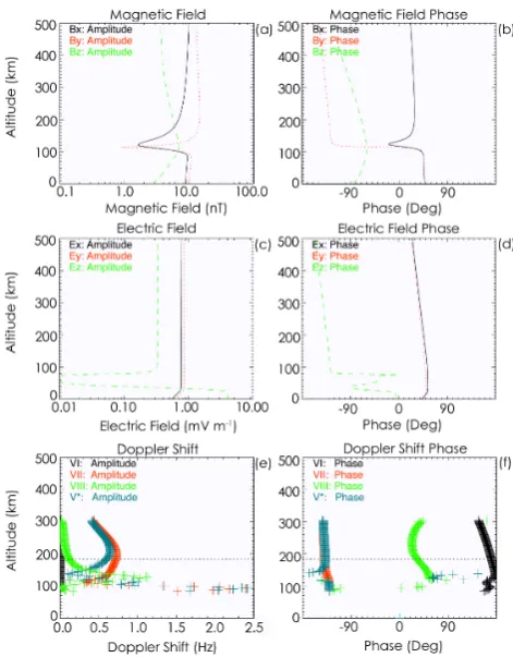
Panels (a) to (d) of Fig. 7 present the results of one run of the model for a purely shear Alfvénic incident wave mode. The magnetic and electric fields are scaled such that the total ground magnetic field matched that from observation (roughly 13.5 nT). Panel (a) presents the variation of the three magnetic field components with altitude. Panel (b) shows the magnetic field phase variation for the same three compo-nents. Panel (c) shows the electric field variation for the three field components as a function of altitude. Panel (d) shows the electric field phase for the same three components.
The effect that the ULF wave has upon the DOPE radio waves can be calculated using a model (Poole and Sutcliffe, 1988), as described in subsequent work by Waters et al. (2007). Panel (e) shows the Doppler shift mechanism ampli-tude, as a function of altitude. Black is the magnetic mech-anism contribution (VI). Red is the advection mechanism
contribution (VI I I) and blue is the overall Doppler shift
(V∗=V
I+VI I+VI I I). Panel (f) shows the phase variation for
the same mechanisms as in panel (e) and is colour coded in an identical fashion. The overplotted black dotted line highlights the DOPE reflection altitude, at roughly 184 km. The overall Doppler shift for a purely shear Alfvénic inci-dent wave is dominated by the advection mechanism (VI I) as
there are very small contributions from the other two mecha-nisms. There are also very large E region values of Doppler shift which is a characteristic of these calculations. The large Doppler shift results from the “knee" in the electron density profile corresponding to a transmission frequency of approx-imately 3 MHz at 100 km, as seen in Fig. 6.
As is clear from Figs. 4 and 5, the wave event under study here has a complicated spatial and temporal structure in am-plitude and phase. The 1-D model is too simplistic to repro-duce accurately the details of the phase relationships between the various magnetic and electric field components, but Wa-ters et al. (2007) demonstrated that Doppler amplitudes are predicted well. Accordingly only model amplitude informa-tion is considered in subsequent plots.
For magnetic field amplitudes recorded on the ground by TRO of 10.0 nT and 9.0 nT, in the X and Y components of the field respectively, the overall Doppler amplitude at the DOPE reflection altitude for a purely shear Alfvénic inci-dent wave determined by the model is roughly 0.5 Hz. This is quite comparable with the typical Doppler Shift as found by the DOPE instrument in the centre of the wave event, of approximately 0.3 Hz at 10:14 UT. However, the ULF wave does not show steady state behaviour throughout the event. The amplitudes in DOPE appear to increase as the wave evolves towards an FLR and the relative phase between mag-netometer stations evolves also (see Fig. 5). One factor which strongly influences the predicted Doppler shift is the wave mix of the incoming ULF wave between fast compressional and Alfvénic wave power. Therefore, an investigation of the effect of wave mix is required in order to determine the pre-dicted Doppler shift that best matches observation through-out the evolution of the wave. Figure 8 presents the elec-tric field, magnetic field and Doppler shift mechanism results as functions of altitude for different wave mixes normalised such that there is a total magnetic field magnitude of 1 nT on the ground. A wave mix of 1.00 is a purely shear Alfvénic incoming wave mode whereas a wave mix of 0.0 is a purely fast/compressional incoming wave mode. Panels (a) and (b) show the X and Y components of the electric field respec-tively. Panels (c) and (d) show the X and Y components of the magnetic field respectively. The electric field in the iono-sphere is clearly a strong function of wave mode for a given ground magnetic field signature, and hence so will be the Doppler signature.
[image:9.595.308.544.60.362.2]Figure 8 also presents the corresponding Doppler shift am-plitude variation as a function of incoming wave mix and altitude. These plots show how a variation in the incom-ing Alfvénic wave mix affects the Doppler Shift amplitude.
Fig. 7. Results of one run of the 1-D Numerical Model for a purely shear Alfvénic incident wave mode for an altitude range from the ground to 500 km. Panel (a) presents the variation of the three magnetic field components with altitude. Panel (b) shows the magnetic field phase variation for the same three components. Panel (c) shows the Electric field variation for the three field com-ponents as a function of altitude. Panel (d) shows the electric field phase for the same three components. Panel (e) shows the Doppler shift mechanism contributions as a function of altitude. Black is the magnetic mechanism contribution (VI), red is the advection
mechanism contribution (VI I), green is the compression
mech-anism contribution (VI I I) and blue is the overall Doppler shift
given by the vector addition of the three Doppler shift components (V∗=VI+VI I+VI I I). Panel (f) shows the phase variation for the
same mechanisms as given in panel (e) and is colour coded in an identical fashion. The overplotted black dotted line highlights the DOPE reflection altitude, at roughly 184 km.
Panel (e) shows the magnetic mechanism. Panel (f) shows the advection mechanism. Panel (g) shows the compressional mechanism. Finally, panel (h) shows the overall Doppler shift, (V∗=VI+VI I+VI I I). As the wave mix tends towards a
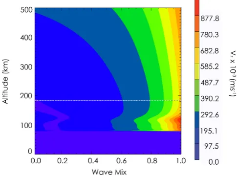
Fig. 8. Electric field, magnetic field and Doppler shift mechanism
results for the ULF wave event on 16 April 1998 between 09:45 UT– 10:45 UT as a function of altitude and wave mix scaled to make the magnetic field magnitude 1 nT on the ground. Panel (a)Ex. (b)Ey. (c)Bx. (d)By. (e)VI. (f)VI I. (g)VI I I. (h)V∗.
DOPE reflection altitude of 184 km, the overall Doppler shift phase looks similar to the “advective" phase.
Panel (a) of Fig. 9 presents the overall Doppler shift vari-ation as a function of wave mix at the DOPE reflection al-titude (184 km), scaled such that we have 1 nT measured on the ground. The scaling allows the determination of the pre-dicted Doppler shift for a given wave mix at different times throughout the event. Matching the observed magnitude of the Doppler amplitudes at various times during the wave event allows the actual wave mode mix to be determined as-sumingkyandkxare constant.
The values of ky, kx and the wave mode mix all affect
[image:10.595.44.291.68.388.2]the overall Doppler magnitude. Eliminating these variables one by one provides an explanation for the model Doppler shifts presented in Fig. 9. Section 3.3 presented a cross phase analysis of the Y components of two azimuthally separated IMAGE stations (TRO and SOR). A constant effective az-imuthal wavenumber was determined, implying a constant east-west wavenumber. ky, therefore, may be neglected as
Fig. 9. Panel (a) shows the overall Doppler shift model results of
the ULF wave event on 16 April 1998 between 09:45 UT–10:45 UT for wave mixes ranging between zero and unity. The panel shows the variation of total Doppler shift with wave mix at the DOPE re-flection altitude of 184 km. Panel (b) presents the variation in the total Doppler shift contributions as a function of altitude andkxThe
overplotted white dashed line shows the DOPE reflection altitude at approximately 184 km. The ground magnetic field in both panels has been scaled to 1 nT.
the cause of variations in the Doppler signature. Thus, the parameter responsible for the nature of Fig. 5 must be either a changing wave mode mix, or the north-south wavenum-ber, kx, or a combination of the two. Panel (b) of Fig. 9
presents the variation in the total Doppler shift contributions similarly to Fig. 8 but now as a function of altitude andkx
for a ground magnetic field magnitude scaled to 1 nT on the ground. Larger Doppler shifts are expected at largerkx
(smaller-scale) values for a given ground magnetic field mag-nitude due to attenuation effects (Hughes and Southwood, 1976a). One would expect an evolvingkx, and an increase
in the X component of the field, as the system tends towards FLR, and this will also affect the total Doppler shift. An analysis of the relative importance ofkxand incoming wave
5 Discussion
Employing the DOPE HF Doppler sounder in conjunction with the IMAGE network of ground magnetometers, the Tromsø dynasonde, the ACE and IMP-8 spacecraft, and a nu-merical model, it is possible to fully characterise the nature of a magnetospheric ULF wave both in the ionosphere and at the ground. The event, which occurred on 16 April 1998, is the result of a low-m (−6) FLR with a large characteristic scale-size. Figure 3 presented the filtered HF Doppler and TRO magnetometer data for the event. The time development of the amplitudes in the Doppler and magnetometer traces was different, with the peak amplitude seen early on in the wave packet in the magnetometer data (10:10 UT), but later in the Doppler trace (10:20 UT). This implies some evolution of the wave characteristics (wave mode, azimuthal or merid-ional scale-size) during the wave. Panel (d) of Fig. 5 showed a phase difference of approximately−60◦between stations TRO and PEL at 10:00 UT evolving to approximately -140◦ at 10:15 UT. The increasing cross phase suggests we have a more FLR-like perturbation as time progresses. Panel (g) of Fig. 2 showed an impulsive disturbance in the solar wind, the effects of which are expected to arrive at the ionosphere be-tween 09:56 UT and 10:07 UT. This impulse is interpreted as the source of the observed wave event.
5.1 Wave evolution
Section 3.3 presented evidence of the model Doppler am-plitude being a result of either variations in kx and/or the
incident wave mode mix sinceky remained approximately
constant throughout the event. To determine the relative importance of the wave mode and/or the meridional scale-size on the Doppler amplitude, ground magnetic field and Doppler observations are used to find inputs to the numeri-cal model at various times throughout the event. The north-south wavenumber may be calculated from the east-west wavenumber and the ratio of the X and Y components of the magnetic field recorded on the ground (Hughes, 1974), which are presented in panels (b) and (c) of Fig. 5. Panel (f) of Fig. 5 presents the north-south wavenumber variation cal-culated from these data. The calcal-culated range ofkx shows
a variation fromkx=1.5×10⁻⁶m-1tokx=3.0×10⁻⁶m-1.
Referring to panel (b) of Fig. 9 it can be seen that such a range ofkx variation has a negligible effect on the derived
total Doppler shift. Therefore, the incoming wave mode mix must be the dominant factor affecting the Doppler amplitude and a constantkx value of 2.1×10⁻⁶m-1 is used in
subse-quent calculations, indicated in panel (f) of Fig. 5 by a hori-zontal red dotted line.
The wave mix variation is calculated by matching the ob-served Doppler shift to the model Doppler shift at 5 min in-tervals throughout the event, which are marked by the verti-cal dotted lines on Fig. 5. At each 5 min interval, the time-evolving Doppler shift, Bx and By are found by using the
DOPE, Bx, and By amplitudes presented in panels (a) to (c) of Fig. 5, respectively. The magnetic field components, therefore, are used to scale the predicted Doppler shift us-ing a constant scale size. Panel (g) of Fig. 5 presents the wave mix evolution derived from such an analysis through-out the event. The first point of the Alfvénic wave mix, at 09:55 UT, has a value of 0.86 (implying contributions from both fast mode compressional and Alfvén modes) although at this time the amplitudes of Doppler shift,BxandByare small so this point is probably not significant. Once the event is es-tablished, at roughly 10:00 UT, the wave mix becomes 0.63 and subsequently rises to unity (a purely shear Alfvén wave) by approximately 10:25 UT. The implied wave mix value of unity occurs just after the peak observed Doppler amplitude as shown in panel (a) of Fig. 5.
5.2 The advection mechanism
The early theory developed by Rishbeth and Garriott (1964) considered that the Doppler frequency oscillations were due to the ULF electric field, causing a vertical bulk motion of electrons in the ionosphere. The vertical motion is the verti-cal component of the plasma drift velocity,
v=(E∧B)Z
B2 . (19)
This vertical motion is now known as the advection mecha-nism. Following Sutcliffe and Poole (1989), the actual con-tribution of this mechanism to the observed Doppler shift is given by
VI I∼= − zR
Z
0
∂µ ∂zVz
dz, (20)
whereµis the real part of the refractive index andzR=zR(t ) is the real height of reflection. BothVzand the vertical
gradi-ent of the refractive index contribute to the observed Doppler shift. The contribution of these two mechanisms may be sep-arated within the model employed here. IfVzis plotted as a
function of both wave mode mix and altitude, assuming the constant value ofkx, and using a magnetic field magnitude
of 1 nT recorded on the ground, Fig. 10 is the result. The very high similarity with the Doppler variation illustrated in panel (f) of Fig. 8 establishes that theVzparameter contained
Fig. 10. The plot showsVzas a function of both altitude and wave
mode mix. The overplotted white dot-dashed line highlights the DOPE reflection altitude at roughly 184 km.
6 Conclusions
In this paper we have employed a numerical one-dimensional model developed by Sciffer et al. (2005) to account for the observed relationship between the Doppler velocity oscilla-tions of reflected radio waves from the ionosphere and ge-omagnetic pulsations. The event that occurred on 16 April 1998 is the result of a low-m (−6) FLR with a large char-acteristic scale-size. An impulsive disturbance is seen in the ACE upstream spacecraft data and the IMF dynamic pres-sure increased at about the same time as the wave onset as recorded on the ground by magnetometers. Here, the effect of the modelled incident wave field on an HF radio path is calculated, and compared to observation. Ground magnetic field and Doppler observations are used to find model in-puts at various points throughout the event. The model, on average, correctly predicts the Doppler amplitudes for this impulse-driven ULF wave event. Presented here, for the first time, are measurements of the wave mode mix evolution. The model demonstrates that the wave mode evolves from a partially Alfvénic wave to a purely shear Alfvén wave. The advection mechanism is contributing the most to the overall Doppler shift at high-latitudes in this instance, agreeing with previous statistical studies of large spatial-scale ULF waves (e.g., Wright et al., 1997, 1998; Waters et al., 2007). For this event it is also confirmed that the vertical velocity dominates the advection mechanism, rather than refractive index effects. 25 ULF wave events with measurements from a high-latitude Doppler sounder and the IMAGE magnetometer array have been analysed. A statistical analysis of large spatial-scale ULF waves will follow this case study.
Acknowledgements. The authors would like to thank the Royal
So-ciety and the STFC for funding the DOPE project. J. D. Borderick
is supported by the STFC. The OMNI data were obtained from the GSFC/SPDF OMNIWeb interface at http://omniweb.gsfc.nasa.gov. The authors also give thanks to the institutes who maintain the IM-AGE magnetometer array.
Topical Editor I. A. Daglis thanks W. J. Hughes and another anonymous referee for their help in evaluating this paper.
References
Allan, W., Poulter, E. M., and White, S. P.: Hydromagnetic wave coupling in the magnetosphere - Plasmapause effects on impulse-excited resonances, Planet. Space Sci., 34, 1189–1200, 1986. Allan, W., White, S., and Poulter, E. M.: Impulse-excited
Hy-dromagnetic Cavity and Field-line Resonances in the Magneto-sphere, Planet. Space Sci., 34, 371–385, 1986b.
Armstrong, T. P., Krimigis, S. M., and Lepping, R. P.: Magne-tosheath burst of predominatly medium nuclei observed with IMP 8 on February 16, 1974, J. Geophys. Res, 83, 5198–5206, 1978.
Bennett, J. A.: The relation between group path and phase path, J. Atmos. Terr. Phys., 29, 893–896, 1967.
Chen, L. and Hasegawa, A.: A Theory of Long-period Magnetic Pulsations, 1. Steady State Excitation of Field Line Resonances, J. Geophys. Res., 79, 1024–1032, 1974a.
Chen, L. and Hasegawa, A.: A Theory of Long-Period Magnetic Pulsations 2. Impulse Excitation of Surface Eigenmode, J. Geo-phys. Res., 79, 1033–1037, 1974b.
Davies, K.: Doppler studies of the ionosphere with vertical inci-dence, Proc. Inst. Rad. Engng, 50, 94–95, 1962.
Davies, K., Watts, J. M., and Zacharisen, D. H.: A Study of F2-Layer Effects as Observed with a Doppler Technique, J. Geo-phys. Res., 67, 601–609, 1962.
Georges, T. M.: Ionospheric effects of atmospheric waves, ESSA Technical Report IER 57-ITSA 54, US Department of Com-merce., 1967.
Hedin, A., Biondi, M., Burnside, R., and Hernandez, G.: Revised global model of thermosphere winds using satellite and ground-based observations, J. Geophys. Res.-Space Physics, 96, 7657– 7688, 1991.
Hughes, W. J.: The Effect of the Atmosphere and Ionosphere on Long Period Magnetospheric Micropulsations, Planet. Space Sci., 22, 1157–1172, 1974.
Hughes, W. J. and Southwood, D. J.: An Illustration of Modifica-tion of Geomagnetic PulsaModifica-tion Structure by the Ionosphere, J. Geophys. Res., 81, 3241–3247, 1976a.
Hughes, W. J. and Southwood, D. J.: The screening of micropulsa-tion signals by the atmosphere and ionosphere, J. Geophys. Res., 81, 3234–3240, 1976b.
Khan, H. and Cowley, S. W. H.: Observations of the response time of high-latitude ionospheric convection to variations in the interplanetary magnetic field using EISCAT and IMP-8 data, Ann. Geophys., 17, 1306–1335, doi:10.1007/s00585-999-1306-8, 1999.
King, J. H. and Papitashvili, N. E.: Solar wind spatial scales in and comparisons of hourly WIND and ACE plasma and magnetic field data, J. Geophys. Res., 110, 1–8, 2005.
Kivelson, M. G. and Southwood, D. J.: Coupling of global magne-tospheric MHD eigenmodes to field line resonances, J. Geophys. Res, 91, 4345–4351, 1986.
Kivelson, M. G., Etcheto, J., and Trotignon, J. G.: Global compres-sional oscillations of the terrestrial magnetosphere: the evidence and a model, J. Geophys. Res., 89, 9851–9856, 1984.
Lee, D.-H. and Lysak, R. L.: Magnetospheric ULF Wave Coupling in the Dipole Model: the Impulsive Excitation, J. Geophys. Res, 94, 17097–17103, 1989.
Luhr, H.: The IMAGE magnetometer network, STEP International Newsletter, 4, 4–6, 1994.
Matsushita, S. and Saito, T.: Geomagnetic pulsations associated with sudden commencements and sudden impulses (Morpho-logical behavior of damped type geomagnetic pulsations associ-ated with storm sudden commencements and sudden impulses), Planet. Space Sci., 15, 573–587, 1967.
Peredo, M., Slavin, J., Mazur, E., and Curtis, S.: Three-dimensional position and shape of the bow shock and their variation with Alfvénic, sonic and magnetosonic Mach numbers and interplan-etary magnetic field orientation, J. Geophys. Res.-Space Physics, 100, 7907–7916, 1995.
Poole, A. and Sutcliffe, P.: The Relationship Between ULF Geomagnetic Pulsations and Ionospheric Doppler Oscillations: Derivation of a Model, J. Geophys. Res., 93, 14656–14664, 1988.
Rishbeth, H. and Garriott, O.: Relationship between simultaneous geomagnetic and ionospheric oscillations, Radio Sci., 68D, 339– 343, 1964.
Samson, J.: Geomagnetic pulsations and plasma waves in the Earth’s magnetosphere, in: vol. 4, London: Academic Press, edited by: Jacobs, J. A., 481–592, 1991.
Sciffer, M. D. and Waters, C. L.: Propagation of ULF waves through the ionosphere: Analytic solutions for oblique magnetic fields, J. Geophys. Res., 107, 1297–1310, 2002.
Sciffer, M. D., Waters, C. L., and Menk, F. W.: A numerical model to investigate the polarisation azimuth of ULF waves through an ionosphere with oblique magnetic fields, Ann. Geophys., 23, 3457–3471, doi:10.5194/angeo-23-3457-2005, 2005.
Siebert, M.: Geomagnetic Pulsations with Latitude-Dependent Pe-riods and their Relation to the Structure of The Magnetosphere, Planet. Space Sci., 12, 137–147, 1964.
Southwood, D. J.: Some Features of Field Line Resonances in the Magnetosphere, Planet. Space Sci., 22, 483–491, 1974. Stone, E. C., Frandsen, A. M., Mewaldt, R. A., Christian, R. E.,
Marglies, D., Ormes, J. F., and Snow, F.: The Advanced Compo-sition Explorer, Space Sci. Rev., 86, 1–22, 1998.
Sutcliffe, P. and Poole, A. W. V.: Ionospheric Doppler and electron velocities in the presence of ULF waves, J. Geophys. Res, 94, 13505–13514, 1989.
Tamao, T.: Transmission and Coupling Resonance of Hydromag-netic Disturbances in the Non-uniform Earth’s Magnetosphere, Sci. Rep. Tohoku Univ., Ser. 5, 17, 43–72, 1965.
Titheridge, J. E.: Ionogram Analysis with the Generalized Pro-gram POLAN, Report UAG-93, World Data Center A for Solar-Terrestrial Physics, US Dept. of Commerce, Boulder. CO 80301, USA., pp. 1–189, 1985.
Voelker, H.: Observations of geomagnetic pulsations: pc 3, 4 and Pi 2 at different latitudes, Ann. Geophys., 24, 245–252, 1968. Waters, C. L.: Corrections to Equations in: A numerical
model to investigate the polarisation azimuth of ULF waves through an ionosphere with oblique magnetic fields, http: //plasma.newcastle.edu.au/~colin/ionosn/eqn_corrections.pdf, Last Checked: 20 July 2010, 2006.
Waters, C. L., Yeoman, T. K., Sciffer, M. D., Ponomarenko, P., and Wright, D. M.: Modulation of radio frequency signals by ULF waves, Ann. Geophys., 25, 1113–1124, doi:10.5194/angeo-25-1113-2007, 2007.
Wright, D. M. and Yeoman, T. K.: High-latitude HF Doppler obser-vations of ULF waves: 2. Waves with small spatial scale sizes, Ann. Geophys., 17, 868–876, doi:10.1007/s00585-999-0868-9, 1999.
Wright, D. M., Yeoman, T. K., and Chapman, P. J.: High-latitude HF Doppler observations of ULF waves. 1. Waves with large spatial scale sizes, Ann. Geophys., 15, 1548–1556, doi:10.1007/s00585-997-1548-2, 1997.
Wright, D. M., Yeoman, T. K., and Davies, J. A.: A compari-son of EISCAT and HF Doppler observations of a ULF wave, Ann. Geophys., 16, 1190–1199, doi:10.1007/s00585-998-1190-7, 1998.
Yeoman, T. K., Lester, M., Orr, D., and Luhr, H.: Ionospheric boundary conditions of hydromagnetic waves: the dependence on azimuthal wave number and a case-study, Planet. Space Sci., 38, 1315–1325, 1990.
Yeoman, T. K., Wright, D. M., and Chapman, P. J.: High-latitude observations of ULF waves with large azimuthal wavenumbers, J. Geophys. Res., 105, 5453–5462, 2000.