The Thirty-Third AAAI Conference on Artificial Intelligence (AAAI-19)
Algorithms for Average Regret Minimization
Sabine Storandt,
1Stefan Funke
21University of Konstanz, Germany,2University of Stuttgart, Germany [email protected], [email protected]
Abstract
In this paper, we study a problem from the realm of multi-criteria decision making in which the goal is to select from a given setSofd-dimensional objects a minimum sized subset
S′with bounded regret. Thereby, regret measures the unhap-piness of users which would like to select their favorite ob-ject from setS but now can only select their favorite object from the subsetS′. Previous work focused on bounding the maximum regret which is determined by the most unhappy user. We propose to consider the average regret instead which is determined by the sum of (un)happiness of all possible users. We show that this regret measure comes with desir-able properties as supermodularity which allows to construct approximation algorithms. Furthermore, we introduce the re-gret minimizing permutation problem and discuss extensions of our algorithms to the recently proposed k-regret measure. Our theoretical results are accompanied with experiments on a variety of inputs withdup to 7.
Introduction
There are numerous (web) services in which it is impossible to present all available options to the user at once; for ex-ample, the list of matching pages in a web search, or the list of products of a certain type in an online warehouse. Hence there needs to be a preselection of a concise subset of the op-tions to be shown to the user first (e.g., on page 1). A typical approach to make this selection is to rank all options using a multivariate function (e.g., for products weighting price, quality, date of appearance, and sales volume) and then pre-senting the top qoptions according to this function to the user. The hope is that the function captures the preference of a typical user or the majority of users. But in case user preferences are diverse, considering only a single function might be insufficient. As a remedy, an alternative selection approach based onregrettakes the preferences of all (pos-sible) users into account. The regret induced by a user pref-erence expressed as a multivariate functionf (to be maxi-mized) with respect to the full set of optionsSand a subset
S′thereof is
1−maxs∈S′f(s)
maxs∈Sf(s)
.
Copyright c⃝2019, Association for the Advancement of Artificial Intelligence (www.aaai.org). All rights reserved.
So in case the best option inS according to the user pref-erence is also contained inS′the regret is 0. In general, the
regret value can assume any value in[0,1].
In previous work, the goal usually was to identify a con-cise subsetS′ofSwhich exhibits a smallmaximum regret,
that is, a subset that makes the unhappiest user sufficiently happy. In this paper, we propose the usage of theaverage re-gretas a viable alternative. We focus on the scenario where user preference functions are (all possible) convex linear combinations of up todcriteria, and provide novel theoret-ical and practtheoret-ical results for computing subsets with small average regret in this setting.
Related Work
The notion of maximum regret as a measure for subset qual-ity was introduced in (Nanongkai et al. 2010) in the context of databases. The idea was generalized to thek–maximum regret measure in (Chester et al. 2014), which does not mea-sure the quality of a subset in relation to the users’ top-1 choice in the whole setSbut to the top-k choice.
It was proven in (Chester et al. 2014) that the problem of computing a subset of given size that minimizes the maxi-mum regret is NP-hard for sufficiently larged. Ford = 2, an exact algorithm based on dynamic programming was pro-posed in (Chester et al. 2014). For largerd, a simple greedy algorithm was discussed in (Nanongkai et al. 2010) and a randomized greedy linear programming algorithm for k -regret in (Chester et al. 2014). Note that both of these greedy algorithms do not come with an approximation guarantee. Known algorithms with an approximation guarantee are ei-ther based on the notion of coresets (Agarwal et al. 2017; Cao et al. 2017; Kumar and Sintos 2018) or by reformulating the problem as a set cover or hitting set problem (Agarwal et al. 2017; Asudeh et al. 2017; Kumar and Sintos 2018). In (Soma and Yoshida 2017), the relation between regret minimization and multi-objective submodular function max-imization was investigated and two algorithms with provable guarantees were proposed.
finite set of possible user utility functions and a probability distribution over these functions. In contrast, we allow an infinite set of utility functions, namely all convex combina-tions ofdcriteria.
Contribution
We motivate and formally define average regret as a measure for the quality of a subset ofd-dimensional objects.
We show that the average regret function is supermodular while the maximum regret function is not. Based on super-modularity, we are able to design a greedy algorithm that computes a subsetS′of given size that comes with a
qual-ity guarantee. And in case we consider the average happi-ness of users, which is defined as 1 minus the average re-gret, we have a submodular function for which we can get a constant-factor approximation algorithm. We show that this even applies in case we consider the more complicated k -regret measure. As a crucial ingredient for the super- and submodular greedy algorithm, we show that the computa-tion of the averagek-regret is possible in time polynomial in
|S|andkfor fixed dimensiond.
In addition, we introduce the average regret minimizing permutation problem, in which the goal is to sort the objects inSsuch that for every prefixs1, . . . , sithe regret is as small
as possible. This allows to smoothly decide for a prefix setS′
with a desired trade-off between size and quality. Moreover, that decision can even be made for each user individually, which allows for more dynamic and customizable services.
Besides theoretical results, we also discuss efficient heuristics for practical use and show their applicability with suitable experiments on a variety of benchmark instances.
Preliminaries
We now provide formal definitions for the average regret measure and the respective optimization problems that will be studied in the paper.
Basic Setting and Properties
We are given a finite set ofd-dimensional objects or points
S ⊂ Rd+ which have non-negative entries in each
dimen-sion. Throughout the paper, we assume the user utility func-tions to be convex linear funcfunc-tions, that is, for some point
s∈Sand some preferenceα∈Rd+with
∑d
i=1αi= 1, we
havef(s, α) =αTs. This is a standard model for user
util-ity functions also used, e.g., in (Soma and Yoshida 2017). Provided with the whole set S, a user chooses the point inS which maximizes his utility function, hence it yields
f(S, α) = maxs∈Sf(s, α) = maxs∈SαTs. As we
as-sume to not know which users will use a service priori, we always consider all possible preferences, that is, all possi-ble α. In a geometric interpretation, the α values form a
d-dimensional simplex. However note that due to the con-straint∑d
i=1αi = 1the valueαdis uniquely defined after
fixing α1, . . . , αd−1. Hence all d-dimensional preferences
are sufficiently described by using a(d−1)-dimensional simplex to which we will refer to asΩ. We will use this ob-servation later to design efficient algorithms.
0 α1 1
SSD RAM
L1
L2
L3
Figure 1: Example for d = 2: Set S consists of three laptops{L1, L2, L3} with different amounts of SSD
mem-ory and RAM (1TB/8GB), (512GB/24GB), (128GB/32GB). The bottom segment in the illustration is the1-dimensional simplex containing all possible values forα1(and implicitly
alsoα2 = 1−α1). The happiness volume induced bySis
the area marked green and blue. For the subsetS′ ={L
3}
the happiness volume is the blue area. The ratio of those two is0.566, leading to an average regret of1−0.566 = 0.434.
We are now ready to formally define the average regret for a subsetS′ of S. Intuitively, we first compute the sum
over all possible utility functionsf(S′, α)which results in a
’happiness volume’ induced by subsetS′. Then we compute
the ’happiness volume’ of the whole setSand divide the for-mer by the latter to get an average happiness or a ’happiness ratio’ in[0,1]which is then subtracted from 1.
Definition 1 (Average Regret) Given a setS and a subset S′ thereof, the average regret ofS′ with respect toS is de-fined asravg(S′, S) = 1−∫Ωf(S′, α)dα/∫Ωf(S, α)dα.
The concept of average regret is illustrated in Figure 1. So why should one use ravg instead of the commonly
applied maximum regret measure rmax(S′, S) = 1 −
minα{f(S′, α)/f(S, α)}?
Assuming the best achievable maximum regret for a sub-set of given size isM, the regret of all other users is com-pletely irrelevant when using the maximum regret measure as long as it is belowM. So while there could be sets where the regret for most users is indeed0, algorithms that mini-mize the maximum regret would not prefer such a solution over one where the regret is exactlyM for all users. The av-erage regret on the other hand would clearly favour a subset in which the regret is small for many users.
In addition, the average regret can be used to lower bound the maximum regret as shown in the following lemma. Lemma 2 ravg(S′, S)≤rmax(S′, S).
Proof. Let B be the maximum regret subtracted from 1,
B = 1−rmax(S′, S) = minα{f(S′, α)/f(S, α)}. Then
we know that for allαit yieldsf(S′, α)/f(S, α)≥Band
hencef(S′, α)≥B·f(S, α). If we plug this into our
for-mula for the average regret subtracted from 1 we get
∫
Ωf(S
′, α)dα
∫
Ωf(S, α)dα
≥B
∫
Ωf(S, α)dα
∫
Ωf(S, α)dα
=B
Optimization Problems
Based on our notion of average regret, we study two related optimization problems in this paper. The first one is the clas-sical problem of computing a subset of fixed size that mini-mizes the regret:
Definition 3 (Regret Minimization Problem) Given a set S, find a subsetS′with|S′|=qsuch that
ravg(S′, S)≤ravg(S′′, S) ∀S′′⊂S,|S′′|=q,
that is, a subsetS′with minimum average regret.
So if on page 1 of a product website there is space forq= 10
objects, a solution to the regret minimization problem con-stitutes a reasonable selection.
However, not in every scenarioqcan easily be determined a priori. For example, a certain website might be viewed on different devices with different screen sizes. On a smart phone, the number of objects that can be viewed at once might be smaller than the number of objects on a tablet, de-manding different values ofq. Moreover, if the user does not like any of the objects shown on page 1, the question is with which objects to proceed on page 2 and so on. This leads to an extended problem formulation:
Definition 4 (Regret Minimizing Permutation Problem)
Given a set S of size n, sort the elements in S such that
∑n
i=1ravg(Si, S)is minimized whereSirefers to the firsti
elements in the sorted list.
We will show that both optimization problems can be tackled with similar techniques.
Modularity and Approximation
In this section, we will exploit the fact that the average regret function ravg(S′, S)exhibits certain characteristics which
allow to design efficient approximation algorithms. More precisely, we will investigate monotonicity, submodularity and supermodularity.
Minimizing Regret and Maximizing Happiness
Remember that the average regret function is defined as
ravg(S′, S) = 1−
∫
Ωf(S
′, α)dα/∫
Ωf(S, α)dα. From now
on we call the subtrahend the average happiness function
havg(S′, S) = 1−ravg(S′, S). Obviously, a subsetS′that
minimizes the average regret automatically maximizes the average happiness. However, that unfortunately doesn’t im-ply that a good approximation algorithm for one of those functions automatically also constitutes a good approxima-tion algorithm for the other funcapproxima-tion, as discussed below.
Submodularity of Average Happiness
For a monotone and submodular set function to be maxi-mized subject to a cardinality constraint on the subset, there exists a simple greedy algorithm that admits a1−1/e
approx-imation guarantee (Fisher, Nemhauser, and Wolsey 1978). So if we can prove that the average happiness function is both, monotone and submodular, we can identify in poly-nomial time a subsetS′ of given sizeqwhich exhibits an
average happiness which is at least1−1/etimes the average
happiness of the optimalq-sized subset.
Definition 5 (monotone) A set function f : 2S →
R is monotone ifA⊂B⊂Simpliesf(A)≤f(B).
Lemma 6 havg(S′, S)is monotone.
Proof. havg(S′, S) =
∫
Ωf(S′, α)dα/
∫
Ωf(S, α)dα. The
denominator is fixed for a given setS. LetS′′ ⊃ S′ be a
superset ofS′. Asf(S′, α) = max
s∈S′αTsit clearly yields
f(S′, α)≤f(S′′, α)as the additional points inS′′\S′can
only increase the function value.
Intuitively, a set function is submodular if the gain of adding an element to a setAis always at least as large as the gain of adding the same element to a superset ofA.
Definition 7 (submodular) A set functionf : 2S →
Ris
submodular if ∀A ⊂ B ⊂ S and s ∈ S \B we have
f(B+s)−f(B)≤f(A+s)−f(A).
Lemma 8 havg(S′, S)is submodular.
Proof. We prove that for each α we have
f(A +s, α)− f(A, α) ≥ f(B +s, α)− f(B, α) for allA⊂Busing a case distinction. In the first case,sdoes not uniquely determine the function value forB+s. Then we have f(B +s, α) = f(B, α)and hence the right side of the submodular inequality becomes0, making it always true. In the second case,suniquely determines the function value for B +s but not forA+s. This is impossible as then we would havef(A+s, α) < f(B+s, α) = αTs
whileαTswould also be a valid function value forA+s. In
the third case,suniquely determines the function value for
B+sandA+s. Then we havef(A+s, α) =f(B+s, α)
which allows to rearrange the submodular inequality to
−f(A, α) ≥ −f(B, α) ⇔ f(A, α) ≤ f(B, α)which is true asf is monotone.
According to those two lemmas, we can use the greedy framework described in (Fisher, Nemhauser, and Wolsey 1978) to find a subset with a constant factor guarantee on the average happiness. The greedy algorithm starts withS′ =∅
and proceeds by iteratively adding the element toS′which
increases the function value the most. After q rounds, the desired subset is found.
Corollary 9 The greedy algorithm computes a fixed size subset ofS which exhibits at least(1−1/e)of the average
happiness of the optimal such subset.
But how does this approximation guarantee for average hap-piness translate to the average regret function?
Theorem 10 A1−1/eapproximation algorithm for optimal
average happinesshprovides a1 + h
e(1−h) approximation
for the optimal average regret.
Proof.Let the average regret be denoted byr= 1−h, we want to upper bound the ratio 11−−ph·h forp= 1−1/eto get the approximation guarantee forrwhile having an approxi-mation guarantee ofpforh. We get:
1−p·h
1−h = 1 +
h(1−p)
1−h = 1 +
h·1/e 1−h
Corollary 11 Forh≤1/2, the approximation guarantee for
the average regret is bounded by1 +1/e.
According to the corollary, forhsmall enough, we get a suf-ficiently strong approximation guarantee forr. But with the average happiness converging to1the approximation factor forrbecomes arbitrarily large.
Supermodularity of Average Regret
A functionfis supermodular if and only if−fis submodu-lar. Equivalently, the following definition applies.
Definition 12 (supermodular) A set functionf : 2S →
R is supermodular if ∀A ⊂B ⊂S ands∈ S\Bwe have f(B+s)−f(B)≥f(A+s)−f(A).
Lemma 13 ravg(S′, S)is supermodular.
Proof.We have shown in Lemma 8 thathavgis submodular.
Therefore, −havg is supermodular. Adding any constant
term does not invalidate the supermodularity. In conclusion,
1−havg=ravgis supermodular.
To demonstrate that this characteristic crucially depends on our regret definition, we now provide a counter-example for supermodularity of the maximum regretrmaxby
demon-strating that1−rmaxis not always submodular.
Example 14 We consider the function
g(S, S) = 1−rmax(S′, S) = min α {f(S
′, α)/f(S, α)}.
To disprove submodularity, we have to find sets A and B with A ⊂ B, such that adding an element s ∈ S \ B to B increases the function value more than it does for A. We use the following example for d = 2: S =
{(6,1),(2,2),(1,6)}, B = {(6,1),(2,2)},A = {(2,2)} ands= (1,6). This leads tog(B) = 1/3(forα= (0,1)), g(A) = 1/3(forα= (1,0)andα= (0,1)) andg(B+s) = g(S) = 1(B +s now equalsS),g(A+s) = 1/3 (for α = (0,1)). Hence we getg(B +s)−g(B) = 2/3 ≥ g(A+s)−g(A) = 0which contradicts submodularity.
So for1−rmaxwe can not easily design a constant factor
approximation greedy algorithm as we did for the average happiness function. And we can also not apply existing re-sults for supermodular functions (Zeighami and Wong 2016) tormaxwhile we can indeed use them forravg. In particular,
we get the following guarantee when using areverse greedy algorithm, which starts with S′ = S and then in each of n−qmany rounds deletes the element whose removal in-creases the average regret the least:
Lemma 15 The reverse greedy algorithm provides an ap-proximation guarantee of(et−1)/tfor the average regret
minimization problem wheret=x/(1−x)withxbeing the steepness ofravg(S′, S).
Here steepness refers to the maximum possible decrease of
ravg(S′, S) when removing an element from S′. The
de-crease is most profound when the element is the only ele-ment inS′. Hence we getx= max
s∈S
∫
Ωf({s}, α)dα.
Regret Minimizing Permutations
One drawback of using the regret minimization problem for subset selection is that the solution is only valid for the par-ticular choice ofq(the subset size). In contrast, the classical ranking method (using only a single mutivariate function) produces a total order of the elements. Hence once the or-der is obtained, a solution for anyqis available by simply outputting the top-qelements in that order.
We now aim for the same level of flexibility when using the regret measure. For that purpose, we want to solve the
average regret minimizing permutation problem. Here, the goal is to compute an ordering of the elements in S, such that the average regret is as small as possible for every prefix
Si. More precisely, we want to minimize the accumulated
average regret over allSifori= 1, . . . , n=|S|. We refer
to the individual regrets asriand to the accumulated regret
asR=∑n
i=1riwithR∈[0, n]. Obviously, it always holds
rn = 0asSn =S, andri ≥ri+1for alli= 1, . . . , n−1
due to monotonicity. Similarly, we define hi = 1−ri as
the average happiness of set Si, andH = ∑ni=1hi as the
accumulated happiness with hn = 1 andhi+1 ≥ hi for
alli= 1, . . . , n−1. Maximizing the accumulated average happiness yields a solution that minimizes the accumulated average regret and vice versa.
We observe that applying the same greedy algorithm we used for the regret minimization problem, also yields prov-ably good solutions for the permutation problem:
Theorem 16 The greedy algorithm yields a1−1/e
approx-imation guarantee for the accumulated average happiness.
Proof.We setq =nand use the order in which the greedy algorithm selects the elements as the desired permutation of
S. Now we know that for any fixedq, the elements selected so far exhibit an average happinesshqof at least(1−1/e)h∗q
where h∗
q is the optimal average happiness achievable for
a subset of size q, see Corollary 9. Hence we can lower boundHas follows:H =∑n
i=1hi ≥∑ni=1(1−1/e)h∗q =
(1−1/e)∑ni=1hq∗ = (1−1/e)H∗whereH∗is the optimal accumulated average happiness.
In the same way, the approximation guarantee for the aver-age regret when using the reverse greedy algorithm (Lemma 15) transfers to the accumulated average regretR.
Average Regret Computation
Although we have proven in the last section that the greedy algorithm is a useful tool for average happiness and average regret computation, there is still one crucial ingredient miss-ing to make the algorithm work: We need to be able to deter-mine the next-best element efficiently, that is, the element in
S whose addition toS′ increases the average happiness the
most in the standard greedy algorithm, or the element inS′
whose removal increases the average regret the least in the reverse greedy algorithm. This demands suitable algorithms to compute∫
Ωf(S
′, α)dα. We will now show that for fixed
dimensiond, this is always possible in polynomial time.
Computing the Happiness Volume
U
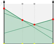
Figure 2: Volume computation ford= 2. We are interested in the green area defined by the upper envelope of the green lines. Via dualization we determine the vertices of the upper envelope (red boxes). We then compute the volume in two steps: We first determine the the volume of the convex hull of the yellow and gray (shadow) vertices, and then subtract from it the volume of the convex hull of the red and gray vertices (gray area) to finally obtain the green area.
practice. To compute the happiness volume for a setS⊂Rd+
of points,|S|=n, we first construct respective hyperplanes
Hin the spaceR+×Ω. More precisely, for each pointp= (p1, p2, . . . , pd)∈S, we create the hyperplane
hp:y= (p1−pd)x1+· · ·+ (pd−1−pd)xd−1+pd.
Additionally, for some very large valueM auxiliary hyper-planesy=M xi,∀i= 1, . . .(d−1)and
y=
(d−1
∑
i=1
M xi
)
−M
are created, which essentially restrict our focus of interest to the positive orthant with∑d−1
i=1 xi ≤ 1. We are interested
in the volume between the hyperplaney = 0and the upper envelope of the hyperplanes.
Since implementations of direct upper envelope construc-tions in dimensions higher than3 are quite rare, we make use of a well-known duality between the upper envelope of an arrangement of hyperplanes and the upper convex hull of respective dual points1. We dualize each hyper-plane h : y = α1x1+α2x2+. . . αd−1xd−1 +αd to a
pointD(h) := (α1, α2, . . . , αd−1,−αd) ∈ Rd. There is a
one-to-one correspondance between the upper envelope of
H and the boundary of the upper convex hull of its dual point set D(H) = {D(h) : h ∈ H}. So we compute the convex hull of D(H), which can be done in expected
O(nlogn+n⌊(d)/2⌋), e.g., via (Clarkson and Shor 1989).
Then every (d −1)-dimensional facet of the upper con-vex hull ofD(H)corresponds to a vertex of the upper en-velope (there are at mostO(n⌊d/2⌋)of them according to
the upper bound theorem (McMullen 1970)). Then for each constructed vertex (α1, α2, . . . , αd−1, y) of the upper
en-velope, we construct its ’shadow’ vertex with coordinates
(α1, α2, . . . , αd−1, U)for some large but fixedU. The
re-sulting vertex set of size O(n⌊d/2⌋) is in convex position,
computing a decomposition of its convex hull into simplices
1
The d transformation does not work for vertical planes, hence the formulation of the auxiliary hyperplanes via some largeM.
can be done inO(nd2/4
). By summing up the volumes of the simplices we compute the volume ’above’ the upper enve-lope. By subtracting it from the volume between the shadow vertices and their counterpart in the hyperplaney = 0we obtain the volume below the upper envelope. See Figure 2 for an illustration.
The total running time isO(nd2/4). In practice, we expect
the complexities of the occurring convex hulls to be consid-erably smaller than in the worst-case, though.
Sampling-based Heuristic
Nevertheless, for higher dimensions or very large point sets the running times for computing the exact volume as above become prohibitive. In that case, a sampling-based approach can be employed which essentially discretizes the param-eter space Ω. So for a given ϵ > 0, we consider the set of points P := (k1ϵ, k2ϵ, . . . , kdϵ) :ki∈N,∑ki= 1/ϵ.
Clearly,|P|=O(ϵ−(d−1)). To approximate the volume
be-low the upper envelope, we simply multiply for eachα∈ P
the volume of a(d−1)-dimensional cube of side lengthϵ
withmaxs∈SαTs. The running time for such an
approxi-mate volume approximation is then O(nϵ−(d−1)). Clearly,
the smallerϵ, the better the approximation.
Extension to
k-Regret
The k-regret measure was introduced in (Chester et al. 2014). The idea is to not measure the quality of a subset
S′for a given preferenceαwith respect to the best element
inSbut to the kthbest element in there. In case the
func-tion value forS′ exceeds the one forSunder this measure
(which is impossible fork= 1but could happen fork≥2), it is capped at the value forS. Then again, thek-regret value can only assume values within[0,1].
We now discuss how averagek-regret works in distinc-tion to the maximumk-regret measure discussed in (Chester et al. 2014). Again, we need the reference happiness volume forS and then the happiness volume forS′to measure the
quality ofS′. Fork= 1, the computations of those two were
independent. But fork≥2, we have to take care of capping the volume of S′ appropriately in case the happiness of a user is larger than the happiness induced by thekthbest
el-ement fromS. We now refer to the happiness volume of the
kthbest elements inS asV
k and to the standard happiness
volume ofS′asV′. Then the averagek-regret is defined as
r(k)
avg= 1−(V
′∩V
k)/Vk.
Figure 3 illustratesVkandV′∩Vkfor an example instance.
Exact Volume Computation Even in case of the general-ization to k-regret, the respective volume computation can actually be done in polynomial time: As in thek = 1case, we first derive the setHof hyperplanes, but then compute the full arrangements of hyperplanes, which can be done in timeO(nd). We then traverse the arrangement, marking all
cells below the k−level and below the hyperplanes inS′.
This can be done in time linear in the complexity of the ar-rangement, henceO(nd). The volume of each of the marked
Figure 3:k-regret ford= 2. The left image shows thekth
best element in each direction among a set of 5 elements and the induced happiness volume fork= 1(green),k= 2
(red),k= 3(blue),k = 4(purple) andk = 5(black). The right image illustrates the hapiness volume (orange area) for a subsetS′consisting of the two orange lines fork= 2. The
area can never include points above the red line.
volumes are easily computed. Clearly, the overall running time is again polynomial, yet we do not consider this ap-proach useful in practice.
Heuristic The above described sampling heuristic trans-lates also to the generalk-regret case by multiplying the vol-ume of the(d−1)-dimensionalϵ-cube with thekthhighest
function value inS, and the best function value in the setS′
(possibly capped at thekthhighest function value inS).
Experiments
We implemented the proposed algorithms for average re-gret in C++, using CGAL 4.11 for computing convex hulls and Eigen 3.3.4 for determining volumes. Experiments were conducted on an AMD Ryzen 2400G with 3.6GHz and 64GB RAM. For benchmarking, we use a variety of differ-ent inputs with the following characteristics:
RC Random points in the unit hypercube (synthetic). We generated up ton= 106points fordfrom 3 to 6.
ElNino Oceanographic data (real-world). It has n = 178080 points for d = 5 (zonal and meridional wind speed, water and surface temperature, relative humidity).
AirData Flight statistics (real-world). It hasn = 458311
points withd= 7(distance, air-time, arr-dely, dep-delay, taxi-out, taxi-in, actual-elapsed-time).
Weather Mean temperatures for every January and July (d= 2) forn= 566262locations around the world.
The real-world data sets were all used before in related pub-lications, e.g., (Soma and Yoshida 2017; Kumar and Sintos 2018). All data sets were normalized to only have values in the interval[1,100]by first subtracting the minimum value in each dimension from the other values in that dimension, and subsequent scaling of the values in each dimension.
Greedy Algorithm: Exact vs Heuristic Selection
We first evaluate the standard greedy algorithm (always adding the next-best element) which has a constant-factor approximation guarantee for the average happiness. We re-port running times and regret values for the exact variant as
exact heuristic d n q ravg time (s) ravg time(s)
3 106 2 0.0014 1462 0.0014 0.54
16 2.2·10−6 1690 0.0006 0.54
3 105 2 0.0019 144 0.0019 0.06
16 5.5·10−6 168 0.0017 0.06 4 105 2 0.0052 603 0.0052 0.20
16 2.6·10−5 1204 0.0007 0.20
4 104 2 0.0060 61 0.0060 0.02
16 0.0002 182 0.0059 0.02 5 104 2 0.0158 274 0.0158 0.05
16 0.0005 3452 0.0116 0.05 5 103 2 0.0101 31 0.0101 0.01
16 0.0002 525 0.0088 0.01 6 103 2 0.0104 113 0.0164 0.01
16 0.0006 15925 0.0141 0.00 6 102 2 0.0504 21 0.0504 0.00 16 0.0008 4190 0.0299 0.00
Table 1: Results for RC with varying values ofn, dandq: exact greedy, and heuristic greedy withϵ= 0.1.
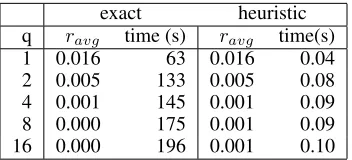
exact heuristic q ravg time (s) ravg time(s)
1 0.016 63 0.016 0.04 2 0.005 133 0.005 0.08 4 0.001 145 0.001 0.09 8 0.000 175 0.001 0.09 16 0.000 196 0.001 0.10
Table 2: Results for the Weather benchmark (d= 2): exact greedy, and heuristic greedy withϵ= 0.1.
well as for the heuristic version, where we estimate the vol-ume of S′+s for alls ∈ S\S′ in each round based on
sampling. To judge the quality of the heuristic greedy truth-fully, we compute the exact happiness volume induced by the final subsetS′.
Synthetic Data For the RC benchmark, the results are summarized in Table 1. For smallq, the average regret values for the exact and heuristic version are the same in almost all settings. Forq= 16, we see that the exact algorithm clearly outperforms the heuristic variant in terms of regret, but at the same time the running times are significantly higher.
Real-world Data For the real-world data sets, the greedy results are collected in Table 2 (Weather), Figure 4 (ElNino) and Table 3 (AirData).
For the Weather benchmark, we observe that the heuris-tic version results in very similar regret values as the exact algorithm, while being faster by up to three orders of mag-nitude. Forϵ≤0.02we even get the very same results from the heuristic and the exact version for all tested values ofq. So in conclusion, the heuristic approach works even better on this real-world data than on our synthetic data.
0 0.005 0.01 0.015 0.02 0.025 0.03 0.035 0.04 0.045
0 10 20 30 40 50 60 70 eps=1/80 eps=1/40 eps=1/10 exact
Figure 4: Average regret in dependency ofqfor the ElNino data set using heuristic greedy with different choices ofϵ.
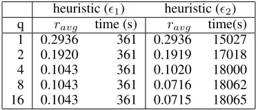
heuristic (ϵ1) heuristic (ϵ2)
q ravg time (s) ravg time(s)
1 0.2936 361 0.2936 15027 2 0.1920 361 0.1919 17018 4 0.1043 361 0.1020 18000 8 0.1043 361 0.0716 18062 16 0.1043 361 0.0715 18065
Table 3: Results for the AirData benchmark (d= 7): heuris-tic greedy withϵ1= 1/20(left) andϵ2= 1/40(right).
the choice ofϵ, see Figure 4. Interestingly, the first elements chosen are always the same regardless of the ϵvalue. But from some value ofqonwards the regret does not decrease anymore. This is due to the sampling based approximate volume computation is not precise enough to reliably de-tect volume increase by different elements anymore. Only a high sampling resolution ofϵ= 1/80leads to regret values close to0. But of course, there is a price to pay: While the algorithm only takes about 2 seconds forϵ= 1/10, it takes almost 3000 seconds forϵ= 1/80.
For the AirData benchmark the exact greedy algorithm was too slow to produce solutions, as the exact volume com-putation becomes expensive with growing dimensiond. But the heuristic version was still applicable. In Table 3, the re-sults for two different choices ofϵcan be found. We observe a similar trade-off between quality and running time as for the ElNino data. The time to select the next point decreases rapidly in both cases.
Standard vs Reverse Greedy
In our theoretical analysis, we exploited two different greedy algorithms: The standard one (always add the next-best el-ement) and the reverse greedy (always remove the element which contributes the least). Both are able to solve the aver-age regret minimization problem for givenqas well as the average regret minimizing permutation problem.
In Figure 5, we compare the two algorithms on an RC benchmark withd = 4andn = 1000. Evidently, the for-ward greedy algorithm outperforms the reverse greedy al-gorithm in all aspects; not only is the accumulated regretR
smaller but also for individual choices ofqup to 30, therq
value is always better. For larger choices ofqthe average
0 0.002 0.004 0.006 0.008 0.01
2 4 8 16 32 64
reverse forward
Figure 5: Average regret in dependency of the subset sizeq
for the standard (forward) greedy algorithm as well as for the reverse greedy algorithm (x-axis in logscale). For the sake of visualization, the plot only starts atq= 2. Forq= 1, the av-erage regret is 0.0107 for the standard greedy and 0.2456 for the reverse greedy algorithm. The accumulated regret over allqisR= 0.0342andR= 0.2790, respectively.
k=1 k=3 k=5 k=7 k=9
q ravg ravg ravg ravg ravg
1 0.3280 0.3161 0.3121 0.3095 0.3016 2 0.2028 0.1949 0.1907 0.1880 0.1790 4 0.0943 0.0901 0.0880 0.0864 0.0772 8 0.0064 0.0018 0.0012 0.0002 0.0001 16 0.0004 0.0002 0.0000 0.0000 0.000
Table 4: Results for the AirData benchmark (d= 7): heuris-tic greedy withϵ = 0.1for different choices ofk, average regret values are based on the approximated volumes.
gret is almost zero for both algorithms. Concerning the run-ning time, the reverse greedy algorithm is slightly slower than the forward algorithm when computing the whole per-mutation (10.7 minutes versus 13.5 minutes). For (small) choices ofq, however, the standard greedy algorithm is way faster as it only requiresqrounds while the reverse greedy algorithm requiresn−qrounds.
Heuristic Computation of Average
k-Regret
Finally, we investigate what happens if we use average k -regret as a quality measure.
Table 4 shows our results on the AirData benchmark for
k = 1,3,5,7,9. Forq = 16running times were between 2 and 3 minutes for all settings. We observe that the average regret decreases with growingkas to be expected. But note that the regret values here are only estimations based on the approximated volume (computed by sampling), as the ex-act volume computation was too expensive even a posteri-ori. Nevertheless it appears that increasingkhas the desired effect on this real-world data set.
Conclusions and Future Work
the heart of our implementation lies the computation of the multi-dimensional happiness volume. For largerd, this is at the moment only possible in a heuristic fashion. In future work, tools from computational geometry should be applied to make the exact greedy algorithm scalable.
References
Agarwal, P. K.; Kumar, N.; Sintos, S.; and Suri, S. 2017. Efficient algorithms for k-regret minimizing sets. arXiv preprint arXiv:1702.01446.
Asudeh, A.; Nazi, A.; Zhang, N.; and Das, G. 2017. Effi-cient computation of regret-ratio minimizing set: A compact maxima representative. InProceedings of the 2017 ACM In-ternational Conference on Management of Data, 821–834. ACM.
Cao, W.; Li, J.; Wang, H.; Wang, K.; Wang, R.; Chi-Wing Wong, R.; and Zhan, W. 2017. k-regret minimizing set: Efficient algorithms and hardness. InLIPIcs-Leibniz In-ternational Proceedings in Informatics, volume 68. Schloss Dagstuhl-Leibniz-Zentrum fuer Informatik.
Chester, S.; Thomo, A.; Venkatesh, S.; and Whitesides, S. 2014. Computing k-regret minimizing sets. Proceedings of the VLDB Endowment7(5):389–400.
Clarkson, K. L., and Shor, P. W. 1989. Application of ran-dom sampling in computational geometry, II. Discrete & Computational Geometry4:387–421.
Fisher, M. L.; Nemhauser, G. L.; and Wolsey, L. A. 1978. An analysis of approximations for maximizing submodular set functions—ii. InPolyhedral combinatorics. Springer. 73– 87.
Kumar, N., and Sintos, S. 2018. Faster approximation al-gorithm for the k-regret minimizing set and related prob-lems. In2018 Proceedings of the Twentieth Workshop on Algorithm Engineering and Experiments (ALENEX), 62–74. SIAM.
McMullen, P. 1970. The maximum numbers of faces of a convex polytope.Mathematika17(2):179–184.
Nanongkai, D.; Sarma, A. D.; Lall, A.; Lipton, R. J.; and Xu, J. 2010. Regret-minimizing representative databases.
Proceedings of the VLDB Endowment3(1-2):1114–1124. Soma, T., and Yoshida, Y. 2017. Regret ratio minimiza-tion in multi-objective submodular funcminimiza-tion maximizaminimiza-tion. InProceedings of the Thirty-First AAAI Conference on Arti-ficial Intelligence, February 4-9, 2017, San Francisco, Cali-fornia, USA., 905–911.