On the construction of approximation space to model discontinuities and cracks with linear and quadratic extended finite elements

R E S E A R C H A R T I C L E

Open Access

On the construction of approximation

space to model discontinuities and cracks

with linear and quadratic extended finite

elements

M. Ndeffo

, P. Massin

, N. Moës

, A. Martin

and S. Gopalakrishnan

*_{Correspondence:}

[email protected]

1_{IMSIA, UMR}

EDF/CNRS/CEA/ENSTA ParisTech 9219, Université Paris Saclay, 828 Boulevard des Maréchaux, 91762 Palaiseau Cedex, France Full list of author information is available at the end of the article

Abstract

This paper presents a robust enrichment strategy to model weak and strong discontinuities as well as cracks for industrial applications. First, numerical issues encountered with popular extended finite element approximation spaces are pointed out. Then, the paper gives indications on how to circumvent those issues. The very originality of the paper relies on questioning the theoretical approximation spaces with respect to numerical results and to modify accordingly their design. The relationship between the new design and the previous designs is clearly established, in order to highlight the very small implementation cost of the modifications exposed here. Hence with minimal additional computational cost, gains in accuracy can be significant as shown later in the paper.

Keywords: Fracture, Quadratic elements, Condition number, X-FEM, GFEM, SGFEM

Introduction

Strain localization is usually an issue for conventional finite element approaches due to numerical issues in the softening regime of the stress–strain relation, when the problem becomes ill-posed. Apart from taking care directly of the localization by an adaptation of the mesh to the discontinuity, different methods have been used in the literature to circumvent this difficulty. Smeared-cracked models were first proposed [1,2] with per-turbations of the fields across the interface. Discontinuous embedded elements appeared almost at the same time with initial papers of Ortiz et al. [3] or Dvorkin et al. [4], with arbitrary orientations through an element but independent from an element to its neigh-bor. A little bit later, special interface elements [5,6] were proposed localized in between conventional elements, which require frequent re-meshing and refined meshes in order to allow for crack propagation in the correct direction. The eXtented Finite Element Method X-FEM [7] and the Generalized Finite Element Method GFEM [8] finally allow meshes not to respect the crack geometry while providing a continuous transfer of information from one element to the next one about the crack surface localization unlike the gener-alized class of embedded discontinuous finite element approaches [3,4]. These methods with nodally based enrichments have managed to combine performance and robustness,

©The Author(s) 2017. This article is distributed under the terms of the Creative Commons Attribution 4.0 International License (http://creativecommons.org/licenses/by/4.0/), which permits unrestricted use, distribution, and reproduction in any medium, provided you give appropriate credit to the original author(s) and the source, provide a link to the Creative Commons license, and indicate if changes were made.

considering non-meshed cracks in a finite element framework. X-FEM and GFEM use the Partition of Unity [9] and enrich the classical basis of shape functions with discontin-uous functions [10]. The discontinuity of the displacement field across the crack surface is then introduced by a generalized Heaviside function, and adding asymptotic fields at the front crack gives good precision in linear elastic fracture mechanics [10,11]. The main advantage of these methods in comparison to mesh-less methods is their easy implemen-tation in a general finite element software, and their capabilities to be applied to various fields: large transformations [12] or plasticity [13] in the X-FEM context for example… One can say that X-FEM and GFEM extend the possibilities of the FEM, while keeping all its advantages. A useful amelioration has been proposed by Sukumar et al. [14] with the introduction of level set functions to represent discontinuities (cracks, voids,…). These approaches are extremely handy in 3D to treat crack propagation [15,16].

Moreover, these methods have been implemented to solve linear elasticity fracture mechanics problems [8,17] with better accuracy than with finite element methods. How-ever, the extension of those methods to quadratic elements in three dimensions is a big challenge. Meanwhile, industrial numerical tools use extensively quadratic elements and simulations in three dimensions are almost the norm. In the wake of [18–20], this arti-cle attempts to close in the gap between the theoretical methods and issues related to implementation in industrial software.

Minor concerns in one dimension with linear elements turn out to be daunting chal-lenges in 3D or with quadratic elements. Those concerns have been described in [17,21– 23] but have raised little interest since recent publications [24,25]. Firstly, they are related to the ill conditioning of strong or weak discontinuous approximations in the general case of non-conforming interfaces and secondly, to the numerical issues related to “geometrical enrichment” techniques, near the crack-tip.

The analysis will be developed more particularly in the case of strongly discontinuous approximations because a direct link with conditioning can be clearly established. For weak discontinuities involved in bi-materials for instance, conditioning issues are still present but they are coupled with the quality of the approximation space to represent continuous solutions with discontinuous gradients [14,26–28]. A specific section will be dedicated to this analysis.

In “Strong discontinuity approximation conditioning” and “Singular enrichment space optimality and conditioning” sections, conditioning issues related to strong discontinuity and singular functions are investigated, as well as, strategies available in the literature to solve those issues. In “Approximation spaces in the literature” and “Numerical behav-ior of strongly discontinuous and singular approximations” sections, those strategies are benchmarked with linear and quadratic elements. Further analysis unfolds that quadratic elements emphasize conditioning and accuracy issues almost unseen with linear elements. The results exposed here are general enough, given the wide range of approximation spaces considered in the paper.

Strong discontinuity approximation conditioning

strate-gies are dependent on the position of the interface or not (see Fig.1). In the literature, the answer is far from obvious. Authors suggested that there is indeed a sensitivity of the solution with respect to the position of the interface; nonetheless, they considered this sensitivity as a numerical side-effect and complex numerical solutions have been elab-orated to deal with this issue [21,24]. Although those techniques may work with linear elements, very little is said about their efficiency with quadratic elements. As a matter of fact, the asymptotic behavior of strongly discontinuous approximations is not well under-stood. Conditioning and accuracy of solutions with strong discontinuities deteriorate severely when the interface gets close to the vertices of the mesh. For curved interfaces or unstructured meshes, the interface has a strong probability of getting close to one vertex at least. Dealing with this configuration is a requirement to prevent unexpected results when switching meshes or when moving the interface during industrial numerical simulations. Those numerical issues have been studied in the case of X-FEM formulations [24]. With X-FEM, the enrichment functions and the classical shape functions are almost collinear when the interface cuts the mesh near one of its nodes (Fig.2). Whenever those config-urations appear, conditioning deteriorates very quickly. In such cases, there are plenty of strategies to limit the condition number large increase. Those strategies are detailed below.

Fig. 1 Positions of the interface investigated in the paper. The condition number is optimal in two cases: firstly, when the interface cuts through the middle of the elements and secondly, when the interface is on the boundary of the elements. Apart from those cases, the condition number soars. This behavior will be investigated later in the paper

First of all, we can consider the elimination of degrees of freedom, based on straightfor-ward criteria [18,24]. Those criteria are rough estimates of the “Heaviside information” on both sides of the discontinuity. Basically, if the Heaviside information is heavily unbal-anced, we have:

– either:

measure+∩Supp(Φi)measure−∩Supp(Φi) (1)

– or:

measure₋∩Supp(Φi)measure₊∩Supp(Φi) (2)

where, Supp(Φi) refers to the support of the shape function and + and − are the domains defined on Fig.3.

Practically, this means that node numberediis either on the side−or on the side+ and does not “see” the information from the opposite side. From now on, the information from the opposite side will be called complementary information.

The criterion used here replaces the measurement of volumes [18,24] by the measure-ment of distances between the nodes of the mesh and the interface on cut edges. When these criteria are associated to a relocation of the interface they are usually named

vertex. Along each edge (see example on Fig.2), the balance of “Heaviside information” is weighted through the comparison of lengths [N1IP] and [N2IP] with respect to [N1N2]. Level-sets (abbreviated “lsn”) are a handy tool to evaluate those lengths, since they do not require computing the coordinates of the intersection points.

From the stand of nodeN1, we have iflsnrefers to the normal level set:

measure(+∩Supp(Φ1)

)∝length([N1IP])≈lsn(N1) (3)

measure(₋∩Supp(Φ1)

)∝length([N2IP])≈lsn(N2) (4)

where N1 and N2are the vertices of the linear element pictured (Fig.2). IP is a given intersection point on the linear element.lsn(x) represents the level-set function at point

x.

Then, the level-set values of both nodes are compared in order to enrich or not node N1. A similar approach consists in changing directly the value of the level-set of the N2 node to zero. In any case, a threshold is needed to decide whether or not the enrichment needs to be modified. This threshold based on the ratio of characteristic dimensions is generally chosen between 10−2and 10−3[18,24].

A simple criterion expresses as:

• Node N1is eliminated or the level set is moved to N2by resettinglsn(N2) to zero if, lsn(N2)

lsn(N1)+lsn(N2)<

10−2 (5)

• Node N2is eliminated or the level set is moved to N1by resettinglsn(N1) to zero if, lsn(N1)

lsn(N1)+lsn(N2)<

10−2 (6)

Apart from distance or volume weighting criteria associated or not to fit-to-vertex, a more evolved criterion may be used [24]. Here, the additional idea is about weighting the “balance of Heaviside information” inside the stiffness matrix, instead of weighting the geometrical information of physical domains. This “stiffness” criterion attempts to correlate the condition number of the “stiffness” matrix to the numerical threshold of elimination.

On second hand, to control the condition number, one can consider an algebraic pre-conditioner [21], dedicated to orthogonalize shape functions and enrichment functions, with a Cholesky factorization.

Let’s assumeKis the stiffness matrix.Ki,xis the term of the matrix associated with shape functionΦiand the enriched d.o.f. corresponding to the enrichment functionFxΦi. As K is bilinear, symmetric and positive definite there is an inner product·,·K such as:

Ki,x= Φi, FxΦiK (7)

Béchet et al. [21] pre-conditioner orthogonalizes Φi andFxΦi (in the sense of·,·K), according to the following procedure:

K →K˜ =P_CTKPC

Ku=f →

˜

Ku˜=PT_Cf

u=PCu˜

(8)

and, ˜

If the degrees of freedom for each node are adjacent (ranked contiguously), the shape of

PCis:

PC =

⎡ ⎢ ⎢ ⎢ ⎢ ⎢ ⎢ ⎢ ⎢ ⎢ ⎢ ⎣

P1_C 0 0 · · · · 0 P2_C 0 · · · 0 · · · 0 0 P3_C · · · ·

· · · . .. · · · · · · · 0 · · · P_Ci · · ·

· · · . .. ⎤ ⎥ ⎥ ⎥ ⎥ ⎥ ⎥ ⎥ ⎥ ⎥ ⎥ ⎦ (10)

The blocks ofPCexpress as follows:

Pi_C =

S_i−1if the node is enriched Id if not

(11)

where the inverse terms are computed from Cholesky’s factorization of local blocks ofK:

K_loci =S_iTSi (12)

K_loci =

⎡ ⎢ ⎢ ⎢ ⎣

Φi,ΦiK Φi, HΦiK Φi, FxΦiK

Φi, HΦi_K HΦi, HΦi_K HΦi, FxΦi_K

Φi, FxΦi_K HΦi, FxΦi_K FxΦi, FxΦiK

⎤ ⎥ ⎥ ⎥

⎦ (13)

Singular enrichment space optimality and conditioning

In linear elasticity, the asymptotic displacement solution at the tip of the crack satisfies (in the local basis defined, Fig.4) [10,11]:

u(r,θ)=

∞

j=0

rλj_kj

1u

j I+k

j

2u

j II+k

j

3u

j III

λj= 1

2 +j (14)

⎧ ⎪ ⎪ ⎪ ⎨ ⎪ ⎪ ⎪ ⎩

u0_I = ₂1_μ2r_πcosθ₂(κ−cosθ)e1+sinθ₂(κ−cosθ)e2

u0_II = ₂1_μ2r_πsinθ₂(2+κ+cosθ)e1+cosθ₂(2−κ−cosθ)e2

u0_III = _μ2₂r_πsinθ₂e3

(15)

where κ = 3−4υ (under the plane strain hypothesis) is Kosolov’s constant andυ is Poisson’s ratio.

The first eigenvalueλ0= 0.5 represents the less regular term of this expansion series. The associated functions (∝√r) are responsible for a significant loss of accuracy within regular FEM [17].

It is the focus point of the X-FEM enrichment to recover at least an order of convergence in energy norm of min (1.5,m), wheremis the interpolation order of the elements (1.5 is related to the regularity of the next eigenvalue λ1). For linear elements, an order of convergence close tom = 1 is expected in the energy norm. For quadratic elements, an order of convergence close tom= 2 is expected in the energy norm, when only the components related to the 0.5 eigenvalue are activated by the boundary conditions.

Laborde et al. [17] showed that a fixed enrichment zone is needed, around the crack-tip, to ensure the optimal accuracy of singular approximations (see Fig.5). This technique uncouples the size of the enrichment zone and the size of the mesh, so that the enrichment zone does not shrink to zero with mesh refinement.

Fig. 4 Plane crack local basis at the crack-tip. Definition of cylindrical coordinates at the crack-tip for plane crack

• The first concern is the definition of the enrichment area and the related enrichment strategy in blending elements. In the literature, two main strategies emerge: the “cut-off” strategy of Nicaise et al. [29] and the geometrical enrichment strategy [17]. Firstly, the “cutoff” strategy adds global singular d.o.f. and an additional function to soften the transition between the enriched zone and the non-enriched zone. Secondly, the geometrical enrichment introduces local singular d.o.f. which values are set to zero outside the enrichment zone. Nicaise and et al. [29] shows that both strategies are relevant and do not alter the convergence rates.

• The second concern is the swift increase of the condition number. Latest works of Chevaugeon et al. [30] and Guptaa et al. [25] give strong research directions to improve the condition number. A vectorial enrichment reduces drastically the number of d.o.f. needed to describe the singular solution. Guptaa et al. [25] suggests that vectorial enrichment could be further improved to permanently remove conditioning issues. The idea of [25] is to subtract from the enrichment function its linear interpolation on the set of elements where the singular enrichment is defined.

Approximation spaces in the literature

In the literature, there are numerous approximation spaces to model strong discontinuities and cracks within the general framework of extended finite element methods and alike. The earliest work of [7] introduced the standard X-FEM approximation space of Table1in 1999. Then in 2000, the work of [8] extrapolated GFEM [22] to crack modeling. Although X-FEM and GFEM both aimed to model cracks, GFEM was designed to deal with a wider scope of problems than X-FEM. Initially, X-FEM and GFEM were assumed as different approaches. X-FEM introduced scalar functions to model Irwin modes at the crack-tip. On the opposite, GFEM used directly Irwin modes as vector functions to model the singular behavior at the crack-tip. In “Approximation spaces for a cracked domain” section, this difference is investigated. We will find out that X-FEM and GFEM are closely related.

In 2004, Laborde et al. [17] paper questioned the numerical accuracy of the X-FEM approximation, particularly with higher order elements. Laborde et al. [17] suggested that X-FEM with one layer of enriched elements at the crack-tip, is not very accurate. When the enrichment zone enlarges, accuracy improves, but conditioning deteriorates. Therefore, it suggested a new approximation space to take care of conditioning issues and with a better behavior for quadratic elements. As this new approximation space is restricted to 2D analysis, this approximation is not fitted for industrial numerical simulations. Finally, to address higher order modeling, X-FEM design evolved into vectorial enrichment [30], close to GFEM.

Very recently, in 2013, even the GFEM approximation space has evolved into a new space called SGFEM [25,31]. SGFEM addresses conditioning issues of GFEM with a new definition of the vectorial functions. Following [32] it is even defined by the fact that the condition number of the associated stiffness matrix has to be of the same order with respect to mesh refinement than the one of FEM. However, SGFEM as proposed in [25,31] has some drawbacks that will be discussed in “Approximation spaces for a cracked domain” section.

jump d.o.f. on nodes in the vicinity of a strongly discontinuous interface (Fig. 3). The next relevant approximation space was the one of Hansbo et al. [33] that introduces discontinuous polynomials within the partition of unity. Numerous spaces were derived from those previous approximation spaces and far too many to be studied thoroughly in this paper [19,20,34,35]. Hence, we will focus, in “Strong discontinuity representation” section, on the ones of Moës et al. [7], Hansbo et al. [33] and Belytchko et al. [36], which is somehow intermediary between those of [7] and [33].

From the mathematical point of view, we will find out that the three spaces are very similar.

Strong discontinuity representation

In this section, we model only a strong discontinuity, with a media fully split by an interface. Hence, we do not need the singular functions in that case. Singular functions will be investigated in the next section.

Thus, let us assume the following X-FEM approximation spaceVh, modeling a strong discontinuity,

Vh=

⎧ ⎨ ⎩uh=

i∈I

aiΦi+

j∈IH

bjHΦj

⎫ ⎬

⎭ (16)

whereΦiare lagrangian polynomials up to order two, in the scope of this article.Idenotes the nodes of the finite element mesh,IH the set of enriched nodes andH the Heaviside function. A node belongs toIH if, and only if, its support is split by the interface. We recall thatHis defined as follows:

∀x∈, x∈/, H(x)=

−1, iflsn(x)<0

+1, iflsn(x)>0 (17) Let’s consider the basic case where the whole domain is divided into two parts as in Fig.3:

• (H=+1)=+ • (H=−1)=−. For which,

• uh₊represents the approximation of the solution on the dimain+extended by continuity to the domain−over the interface,

• uh

−represents the approximation of the solution on the dimain−extended by continuity to the domain₊over the interface.

The representation of the kinematic jump is crucial for many interfacial laws, such as cohesive laws and contact laws. The jump at every point (commonly integration point) located on the interface, follows the convention:

∀x∈, uh(x)=

uh

+− u h

−

(x) (18)

In order to simplify the notations in Table1, we define for a given nodej ∈ IH,j,1 = χ+jandj,2=χ−j, whereχAdenotes the characteristic function of the setA. Using these notations, we have:

Hj−Hxj

j=

+2χ+j= +2j,1, ifj∈−

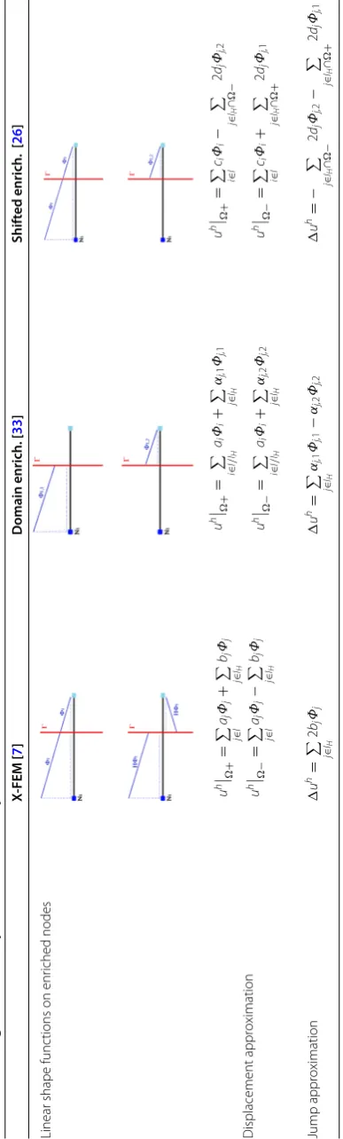
Table 1 Strong discontinuity enrichments comparison X-FEM [ 7 ] D omain enrich. [ 33 ] S hifted enrich. [ 26 ] Linear shape functions on enriched n odes Displacement approximation u h + =

j∈I aj

Φj

+

j∈IH bj Φj u h − =

j∈I aj

Φj

−

j∈IH bj Φj u h + =

_i∈I/I

H

ai

Φi

+

j∈I

H

αj,1

Φj,1

u

h

−

=

_i∈I/I

H

ai

Φi

+

j∈I

H

αj,2

Φj,2

u

h

+

=

i∈I ci Φi − j ∈ IH ∩ − 2 dj

Φj,2

u

h

−

=

i∈I ci Φi + j ∈ IH ∩ + 2 dj

Φj,1

Jump

approximation

u

h= j∈I

H 2 bj Φj u h= j∈I

H

αj,1

Φj,1

−

αj,2

Φj,2

u h=− j ∈ IH ∩ − 2 dj

Φj,2

− j ∈ IH ∩ + 2 dj

Φj,1

wherexj is the location ofj. The functionH−H

xj

is used to define the formulation introduced in [26].

Let us compare side-by-side, the XFEM representation of the displacement jump intro-duced by [7] with the other well-known formulations of [33] and [26]. Even though the jump approximations have different expressions (Table1), we will investigate next whether the approximation spaces are really different or not.

Areias et al. [37] showed that [7] and [33] involve different bases but that both enrich-ments still represent the same approximation space. Each enrichment can be expressed in terms of the other one with a suitable change of variables. With the same analysis as in [37], the different enrichments can be expressed in terms of the other ones for the remaining couple of formulations X-FEM/Shifted and Domain/Shifted.

Thus, from the mathematical point of view, the approximation spaces involved in the three formulations are equivalent (see Table 2). The same can be said of other formu-lations encountered in the literature [19,34,35]. We would like to stress the fact that this equivalency only holds in the case of strong discontinuity. When singular functions are injected in the approximation, the relationship between the different approximation spaces may be different as studied in the next section.

Approximation spaces for a cracked domain

The model problem is a cracked domain(Fig.6), under a linear elasticity assumption. The material is also assumed to be homogeneous and isotropic. Dirichlet boundary con-ditions are applied on the boundaryDand Neumann boundary conditions are applied onN.

The space of admissible displacements is:

V =v∈H1();v=0onD (19)

Table 2 Change of variables when switching enrichment strategies.∀j∈IH, the following

Fig. 6 Example of a cracked domain. Definition of notations used to label the domain and its boundaries

The weak form of the equilibrium problem is:

P:

⎧ ⎪ ⎪ ⎪ ⎨ ⎪ ⎪ ⎪ ⎩

Find u∈V such that a(u, v)=l(v) ∀v∈V,

a(u, v)=σ(u) :ε(v)d,

l(v)=f ·v d+

N g·v d,

σ(u)=λtr(ε(u))1+2με(u),

(20)

whereuis the displacement,σis the Cauchy stress,εis the strain, 1 the identity tensor,f is the body force applied onω,gis the traction applied onN andλandμare the Lamé parameters.

Now, the discrete approximation spaces from the literature will be investigated. In the fol-lowing sections, we will prove that spaces available in the literature can be gathered into two classes: “straightforward” enrichment and “bubble” enrichment. An illustration of those two classes is provided on Fig.7. “Straightforward” enrichment means that the sin-gular function is introduced directly into the approximation space without modification. “Bubble” enrichment means that the singular function is reshaped into a new function before its introduction into the approximation space.

In the following sections, those classes are described:

• “Straightforward” singular enrichment class” section shows that X-FEM and GFEM are “straightforward” enrichments. Moreover, GFEM is a subspace of X-FEM. This statement implies that X-FEM is somehow more accurate than GFEM, but both methods are nonetheless very close.

Fig. 7 “Straightforward” enrichment class versus “bubble” enrichment class. The difference in shape highlights the difference in behavior stated in the previous section

“Straightforward” singular enrichment class

Let Vh be the approximation space using vector asymptotic functions to describe the crack kinematics:

Vh=

vh=_i∈Id_j=1ai,jΦiE_j+_i∈IHd_j=1bi,jHΦiEj

+i∈ICT

d

α=1ci,αΦiK_α

(21)

whered is equal to two in the bidimensional case and three in the tridimensional case,

E₁, E₂, E₃is the usual Cartesian basis,K_αare the vector asymptotic functions andICT the set of nodes enriched by such functions. In this contribution,ICTis defined as the set of nodes placed at a distance lower thanRfrom the crack-tip (cf. Fig.5).

The vector asymptotic functionsK_αare defined as follows:

⎧ ⎪ ⎨ ⎪ ⎩

K₁=u0_I

K₂=u0_II

K₃=u0

III

(22)

withu0_I, u0_II u0_III given by (15).

V_CUTOFFh (W2,∞)=

vh=_i∈Id_j=1ai,jΦiE_j+_i∈IHd_j=1bi,jHΦiEj+ d

α=1cαχKα

(23)

and letV_XFEMh be the standard X-FEM approximation space [7]:

V_XFEMh =

⎧ ⎨ ⎩

vh=_i∈Id_j=1ai,jΦiE_j+_i∈IHd_j=1bi,jHΦiEj+

k∈ICT

α=1,4

_d

j=1c j

k,αFαΦkEj

⎫ ⎬

⎭ (24)

whereFαare defined as:

⎧ ⎪ ⎪ ⎪ ⎨ ⎪ ⎪ ⎪ ⎩

F1=√rsinθ₂

F2=√rcosθ₂

F3=√rsinθ₂sinθ

F4₌√_rcosθ

2sinθ

(25)

We remark that:

_√

rcosθ₂cosθ =F2−F3

√

rsinθ₂cosθ =F4−F1 (26)

Consequently, the vector functionsK_α and the scalar functions Fα are related by the following linear relations:

⎧ ⎪ ⎪ ⎪ ⎨ ⎪ ⎪ ⎪ ⎩

K₁= 1

2μ√2π

(κ−1)F2+F3e1+ 1

2μ√2π

(κ+1)F1−F4e2

K₂= 1

2μ√2π

(κ+1)F1+F4e1+ 1

2μ√2π

(1−κ)F2+F3e2

K₃= 2

μ√2πF1e3

(27)

Lemma 1 V_CUTOFFh (W_h2,∞)is a subspace of Vh and Vh is a subspace of V_XFEMh , i.e. the three approximation spaces are related as follows,

V_CUTOFFh (W_h2,∞)⊂Vh⊂V_XFEMh

where W_h2,∞is the subspace of interpolated cutoff functions.

Proof The proof relies on the work of [29].

• V_CUTOFFh (W_h2,∞)⊂Vh: Forvh∈V_CUTOFFh (W_h2,∞),

vh=

i∈I d

j=1

ai,jΦiE_j+ i∈IH

d

j=1

bi,jHΦiEj+

d

α=1

c_αχhK_α

χhis the interpolation of a cutoff functionχwhich vanishes outsideICT,

χh=

i∈ICT

χ(xi)Φi

Then,

vh=

i∈I d

j=1

ai,jΦiE_j+ i∈IH

d

j=1

bi,jHΦiEj+

i∈ICT d

α=1

c_αχ(xi)ΦiK_α

which leads to,

• Vh⊂V_XFEMh : Forvh∈Vh,

vh=

i∈I d

j=1

ai,jΦiE_j+ i∈IH

d

j=1

bi,jHΦiEj+

k∈ICT d

α=1

ck,αΦkKα

• Equation (27) shows thatK_α can be expressed asK_α = 4 l=1

d

m=1

k_l,m,αFl_em_{, where} ki,m,αis a constant tensor.

In case of a straight crack, the local basis is constant.

Thus, the local basis expresses in cartesian coordinates as,em = d

j=1

μm,jE_j, where μm,jis a constant tensor.

Then,

K_α =

4 l=1 d m=1 d

j=1

k_l,m,αμm,jFlE_j

d

α=1

c_k,αΦkK_α =

d

α=1 4 l=1 d m=1 d

j=1

c_k,αk_l,m,αμm,jFlΦkE_j

=

4

l=1 d

j=1 ⎛

⎝d

α=1 d

m=1

ck,αkl,m,αμm,j

⎞ ⎠FlΦkE_j

With a suitable change of variable,

c_k,lj =

d

α=1 d

m=1

ck,αkl,m,αμm,j

we have finally,

vh=

i∈I d

j=1

ai,jΦiE_j+ i∈IH

d

j=1

bi,jHΦiEj+

k∈ICT 4

l=1 d

j=1

cj_k,lFlΦkE_j

which means that:

vh∈V_XFEMh

• In case of a curved crack, the result of the lemma holds with a discretization of the local basis of [30]. Let us consider a discrete local basis at each nodee1_k, e2_k, e3_k, such as,

vh=

i∈I d

j=1

ai,jΦiE_j+ i∈IH

d

j=1

bi,jHΦiEj+

k∈ICT d

α=1

c_k,αΦkK_α,k

K_α,k=

4 l=1 d m=1

kl,m,αFlemk

em_k =

d

j=1 μm,j,kE_j

The straight crack proof still holds here, with the additional node index “k”.

Remark as a practical consequence of Lemma-1, the error bound of X-FEM should be lower than the ones ofVhand of the cutoff [29]. With X-FEM, the optimization process performs on a larger space than with other formulations and reaches a closer infimum to the exact solution of the problem. Nevertheless, X-FEM introduces more d.o.f. than GFEM and cutoff enrichments which increases its condition number.

“Bubble” enrichment class

Now, let us consider the SGFEM space for linear elastic fracture mechanics similar to the one proposed in [25,31]:

V_SGFEMh =

vh=_i∈Id_j=1ai,jΦiE_j+_i∈IHd_j=14_k=1bi,j,kHψi,kΦiEj

+_i∈ICTd

α=1ci,αΦi

K_α−K_α

(28)

whereψi,k_k=1..4=1, x−xi, y−yi, z−zi

, andK_α =_k∈{I

CT∪δICT}Kα(rk,θk)Φk is

the usual interpolation.

δICTis defined here as the transition layer of nodes between crack-tip elements and other elements of the mesh for whichK_αunknowns are set to zero. This allows to connect the enriched layer with the remaining of the mesh and to avoid blending issues [26].

Lemma 2 V_XFEMh is not a subspace of V_SGFEMh and V_SGFEMh is not a subspace of V_XFEMh , so that:

V_XFEMh ⊂V_SGFEMh and V_SGFEMh ⊂V_XFEMh (29)

Proof – V_SGFEMh ⊂V_XFEMh

It is obvious thatV_SGFEMh ⊂V_XFEMh becauseV_SGFEMh involves higher order discontinuous polynomialsHψi,kΦi, which are out ofV_XFEMh .

– V_XFEMh ⊂V_SGFEMh

• F1_E 1

k∈ICT

Φk belongs to the test function space Vh

XFEM with ai,j = 0, bi,j = 0, c_k,1₁=1 andcj_k,α=0 elsewhere (forα=1).

• However, F1E₁ k∈ICT

Φk does not belong toV_SGFEMh , which can be shown by

contradiction.

• Let us assumeF1E₁ k∈ICT

Φkbelongs toV_SGFEMh ,

F1E₁

k∈ICT

Φk =

i∈I d

j=1

ai,jΦiE_j+ i∈IH

d

j=1 4

k=1

b_i,j,kHψi,kΦiE_j

+

i∈ICT d

α=1

ci,αΦiKα−Kα

• Singular functions cannot be represented by discontinuous polynomials basis, so we necessarily havebi,j,k =0

• Singular functions cannot be represented by continuous polynomials as well, so,

i∈I d

j=1

ai,jΦiE_j− i∈ICT

d

α=1

ci,αΦiK_α=0 asΦiK_αis also a polynomial.

• Which leads to, d

α=1

ci,αΦiKα =0,

• Then,ci,α =0,

• And,ai,j=0 because d

j=1

ai,jΦiE_j =0.

• Thus,F1E₁ k∈ICT

Φk =0 which is contradictory.

Remark As a practical consequence of Lemma-2 the “bubble” class of “Bubble”

enrich-ment class” section does not belong to the “straightforward” class of “Straightforward” singular enrichment class” section, in which X-FEM is found to be the largest space. Hence, the definition of two classes of enrichment makes perfectly sense.

Numerical behavior of strongly discontinuous and singular approximations

In this section the numerical behavior of the different approximation spaces introduced previously is investigated through a couple of benchmarks. First of all, we assess the asymp-totic behavior of strongly discontinuous approximations, through a one dimensional case. Secondly, we consider the convergence study of a two-dimensional problem with a crack and singular approximation.

Numerical behavior of strongly discontinuous approximations

Numerical analysis of strongly discontinuous approximations with linear elements

Let us consider the basic case of the traction of a one-dimensional bar with a fictitious bi-material interface. The arbitrary interface is positioned along the abscissax(ε) (Fig.8). The problem even though continuous is treated as a discontinuous one, with gluing interface boundary conditions imposed through a Lagrange multiplier. Actually, if the materials were different on each side of the interface, the resulting problem would be equivalent to enforcing a weak discontinuity with a strong discontinuity framework. This artefact is used so as to establish convergence results in energy norm. If it was not the case, the solution obtained would be that of two rigid bodies with prescribed displacements on one of their end.

• The problem is the solution of the following differential equation:

u(x)=0 ∀x∈=[0,3] (30)

• With arbitrary Dirichlet boundary conditions:

u(0)=β u(3)=3α+β (31)

• And with continuity conditions at the interface expressed in terms of the continuity of the derivative of the displacement field (stress continuity at the interface):

du dx

x(ε+)

=α− du dx

x(ε−)

=α+ α−=α+=α (32) This continuity condition results from the equivalent Lagrangian form of (30) in which a Lagrange multiplierλis used to impose a continuous displacement across the interface. (u,λ) is the saddle point of the following functional:

L(u,λ)= 1

2 3 $

0

u2dx+λuxε+−uxε−=0

The expected continuous solution satisfying the boundary conditions above, is:

u(x)=αx+β, ∀x∈[0,3] (33)

The resulting weak form of the problem is:

Find,

u∈%:w∈H1/w(0)=β, w(3)=3α+β,λ∈

∀v∈%₀:w∈H1/w(0)=0, w(3)=0

∀μ∈R

⎫ ⎪ ⎬ ⎪ ⎭ → ⎧ ⎪ ⎨ ⎪ ⎩ ₃

0 uvdx=0

λ−α+_vxε+_−λ−α−_vxε−₌₀ μuxε+−uxε−=0

(34)

The X-FEM discrete linear space is:

&

h:

w/w=a11+a22+b2H2+a33+b3H3+a44

a1=β a4=3α+β

(35)

Then, the 6×6 matrix associated with the discretization of the weak form on the X-FEM space of linear functions (first column of Table1) is:

⎡ ⎢ ⎢ ⎢ ⎢ ⎢ ⎢ ⎢ ⎢ ⎣

1 −1 1 0 0 0

−1 2 −2+2ε −1 1−2ε 0

1 −2+2ε 2 1−2ε −1 0

0 −1 1−2ε 2 2ε −1

0 1−2ε −1 2ε 2 −1

0 0 0 −1 −1 1

⎤ ⎥ ⎥ ⎥ ⎥ ⎥ ⎥ ⎥ ⎥ ⎦ ⎧ ⎪ ⎪ ⎪ ⎪ ⎪ ⎪ ⎪ ⎪ ⎨ ⎪ ⎪ ⎪ ⎪ ⎪ ⎪ ⎪ ⎪ ⎩ a1 a2 b2 a3 b3 a4 ⎫ ⎪ ⎪ ⎪ ⎪ ⎪ ⎪ ⎪ ⎪ ⎬ ⎪ ⎪ ⎪ ⎪ ⎪ ⎪ ⎪ ⎪ ⎭ (36)

With the domain formulation of the second column of Table1, the discrete matrix is:

⎡ ⎢ ⎢ ⎢ ⎢ ⎢ ⎢ ⎢ ⎢ ⎣

1 −1 0 0 0 0

−1 2−ε 0 −1+ε 0 0

0 0 ε 0 −ε 0

0 −1+ε 0 1−ε 0 0

0 0 −ε 0 1+ε −1

0 0 0 0 −1 1

With the shifted formulation of the third column of Table1, the discrete matrix is: ⎡ ⎢ ⎢ ⎢ ⎢ ⎢ ⎢ ⎢ ⎢ ⎣

1 −1 0 0 0 0

−1 2 2ε −1 2−2ε 0

0 2ε 4ε −2ε 0 0

0 −1 −2ε 2 −2+2ε −1

0 2−2ε 0 −2+2ε 4−4ε 0

0 0 0 −1 0 1

⎤ ⎥ ⎥ ⎥ ⎥ ⎥ ⎥ ⎥ ⎥ ⎦ ⎧ ⎪ ⎪ ⎪ ⎪ ⎪ ⎪ ⎪ ⎪ ⎨ ⎪ ⎪ ⎪ ⎪ ⎪ ⎪ ⎪ ⎪ ⎩ c1 c2 d2 c3 d3 c4 ⎫ ⎪ ⎪ ⎪ ⎪ ⎪ ⎪ ⎪ ⎪ ⎬ ⎪ ⎪ ⎪ ⎪ ⎪ ⎪ ⎪ ⎪ ⎭ (38)

We enforce boundary conditions directly on the discrete problem, as equality constraints through Lagrange multipliers. The position of the interface depends only onε. Nonethe-less, the solution does not depend on theεparameter, so that the relative error does not depend onε, which makes our analysis relevant.

Let us consider the following arbitrary numerical values:α=10/9 andβ=10. Then, the solution is computed in standard 64-bit arithmetic, with the linear solver UMFPACK, to reproduce the behavior of direct solvers.

The numerical error has to be close to zero, for any given position of the interface. The error is evaluated here in terms of the H1-norm:

u−u_hH1 =

'$ 3

0 (

(u−u_h)2+u−u_h2)dx (39)

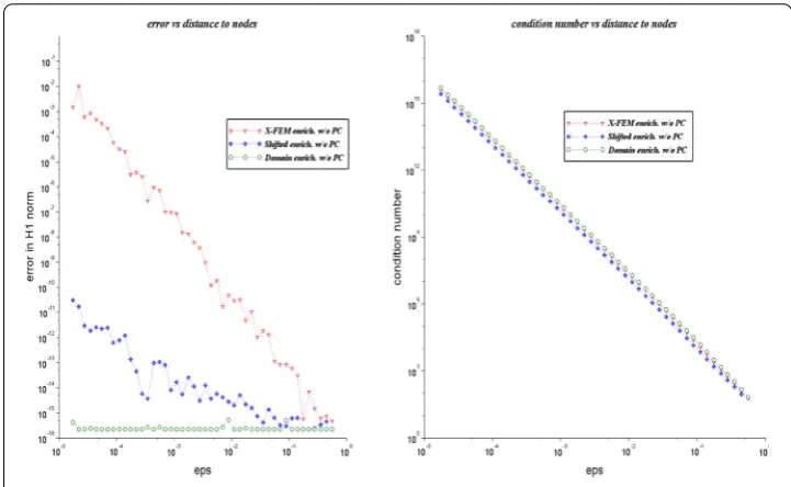
Although all three formulations represent the same approximation space, they do not have exactly the same numerical behavior (Fig.9), at least concerning the error in H1_-norm. The X-FEM error increases steadily while the “shifted” formulation and the “domain” formulation levels of error stay close to machine precision (about 2.2·10−16).

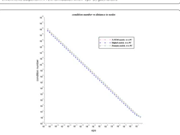
Moreover, all three enrichment conditionings increase as the distance between the interface and node N3decreases (Fig.10). This means that all three enrichment strategies are very sensitive to the position of the interface. A pre-conditioner is needed for the three enrichments. In the case of X-FEM, we studied Béchet et al. [21] pre-conditioner. For other formulations we used a diagonal pre-conditioner to scale the d.o.f.

The diagonal pre-conditioner allows a scaling of rows and columns through a multipli-cation with a diagonal matrix to the left and to the right:

Ku=f →Ku=fwith

⎧ ⎪ ⎨ ⎪ ⎩

K=DcKDc

u=Dcu

f=Dcf

(40)

In linear elasticity,Dcis usually defined as,

[Dc]i,i= 1

*

Ki,i

+

max(Ki,i)+min(Ki,i)

2 (41)

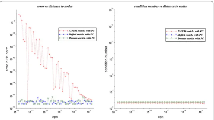
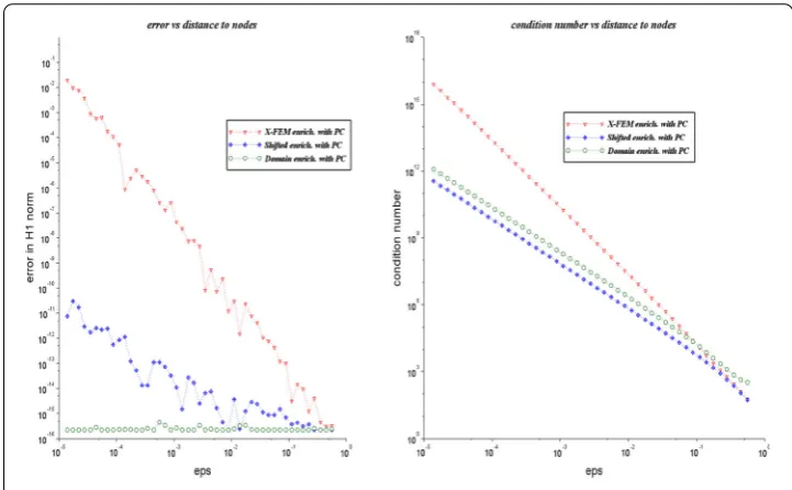
Thus, on Fig. 11, condition numbers are reduced drastically. However, the error still increases in case of X-FEM. The error is clearly not only related to conditioning. Another explanation should be considered.

When looking at the X-FEM discrete stiffness matrix, it is noticeable that the unknowns a2andb2obey to an almost similar equation (asH2 ≈ −2). The difference between those equations lies in the terms 1 −2ε and 2− 2ε. Those terms imply the sum of heterogeneous quantities that leads to a tremendous loss of accuracy on the difference information 2ε. For instance, let us consider the following string of calculations in “double precision” arithmetic (8-octet storage):

Fig. 9 H1-error of strongly discontinuous approximations with linear elements. Shifted and domain enrichments outperform X-FEM formulation when “eps” (ε) goes to zero

Fig. 11 The use of dedicated pre-conditioners improves the condition number but has little effect on X-FEM accuracy. According to the curves above, conditioning and accuracy are clearly two separated issues: improving the condition number does not automatically solve accuracy issues. Conditioning and accuracy are both symptoms of the faulty behavior of partition of unity with asymptotically small domains

The final result 6.348E–12, is quite different from the exact result 6.3487497084E–12: only four digits remain of the “difference information” between the equations. Hence ill conditioning indicates also a lesser accuracy within the assembled stiffness matrix due to round-off errors and truncated information. Even highly effective pre-conditioners [21] cannot recover the truncated information. It is not surprising that, besides precondition-ing, authors have used triple precision arithmetic to recover accuracy [24].

Remark Because the error curves are shattered, the phenomenon might be also

proba-bilistic and related to random round-off errors in interaction with the solver algorithm. A comprehensive study with a wide range of solvers is presented (Figs.12and13). This study shows that the type of solver interferes with the level of error, which makes numerical analysis on errors quite sensitive:

• For iterative methods (PCG), the error is generally higher because those solvers are very sensitive to conditioning,

• For matrix factorization based solvers (UMF), the error is lower than with iterative methods,

• For matrix inversion based solvers, good results can be obtained frequently.

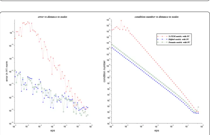
Numerical analysis of strongly discontinuous approximations with quadratic elements The same one-dimensional case is considered here. The same discretization of the weak form is used with quadratic shape functions. The results are plotted on Fig.14.

Fig. 12 Overall error analysis of a wide range of solvers for the 1D case. Only X-FEM’s enrichment without pre-conditioner is studied here. The whole trend suggests a global increase of the sensitivity of solvers (with respect to epsilon), when the “epsilon” parameter goes to zero

Fig. 13 The use of dedicated pre-conditioner stabilizes the behavior of solvers. But the error still increases with the X-FEM method, as explained in “Numerical analysis of strongly discontinuous approximations with linear elements” section

On Fig.15, the same pre-conditioners than in “Numerical behavior of strongly discon-tinuous approximations” section are considered. The wrong behavior noticed above still applies.

This numerical behavior with quadratic elements is well explained by the coupling between enrichment functions, as pictured on Fig.16with domain enrichment [33].

Whenmeasure(+∩Supp(ΦS))→0 for a given vertex node, the middle node

Fig. 14 H1-error and conditioning analysis with quadratic elements (Lagrange). The conditioning slopes are about three as shown is “Numerical analysis of strongly discontinuous approximations with quadratic elements” section

Fig. 15 The use of linear element pre-conditioners barely improves the accuracy and condition number of quadratic elements (Lagrange)

• In case of Lagrange polynomials, we have: ΦS(ξ)=(1−ξ)(1−2ξ), ∀ξ ∈[0,1]

ΦM(ξ)=4ξ(1−ξ), ∀ξ ∈[0,1] (43)

Both functions can be related with the following expression,

Fig. 16 Coupling between Lagrange quadratic shape functions. When the crack passes close to the nodes, the discontinuous shape functions of the middle node and one vertex node become almost colinear

interface

[ ]0,1 1(x) 2₅(1 x)χ

e = −

ε

1 2 3 4 5 6 7

interface

[2 ,2] 2 2(x)= ₁₇4 (2−x) χ −ε

e

1 2 3 4 5 6 7

ε

(a)

(b)

Fig. 17 Graphs of polynomial functionse1(a) ande2(b)

whenξ goes to 1, the difference information between those functions decreases accord-ingly to (1−ξ)2. This generates a vanishing sub-space (consisting of polynomials only defined on the small support ₊∩Supp(ΦS)), which implies a conditioning slope of at least 3 with quadratic shape functions (Fig.15). In other words, the condition number κ(K) is bounded by:

κ(K)≥Cε−3 (45)

Proof Letκ(K) be the condition number of the stiffness matrix:

κ(K)=

maxeT_Ke e2=1

mineT_Ke e2=1

≥ e1TKe1

e₂TKe2 ∀

e1, e2/e12=1,e22=1 (46)

where2is the Euclidian norm 2.

In order to estimate the lower bound of the condition number, we consider the polyno-mialse1ande2illustrated on Fig.17.

e1= −√1₅(21+2)

e2= √1₁₇(4χ−₃+χ−₄) (47)

In the discrete space of [33], we have:

u₂=' i∈I/IH

a2_i +

j∈IH α2

j,1+

j∈IH α2

j,2 (48)

so that we havee12= e22=1.

As 1₂e₁TKe1and1₂eT2Ke2represent the elastic energy of these solutions, we have:

e₁TKe1

e₂TKe2 =

1 0

e₁2dx

2

2−ε

e₂2dx =

51 80ε3

Thus,

κ(K)≥Cε−3

The asymptotic behavior ofΦM(ξ) [at the first order of (1−ξ)] is: ΦM(ξ)≈ −ΦS(ξ)/4

Then, the related d.o.f. become redundant, which leads to ill conditioning. As enrichment strategies are equivalent, the redundant d.o.f. pollutes also the approximation spaces of the other formulations [7,26].

• In case of Bernstein polynomials, we have: ΦS(ξ)=(1−ξ)2, ∀ξ ∈[0,1]

ΦM(ξ)=2ξ(1−ξ), ∀ξ ∈[0,1] (49)

whenξ goes to 1, there is no coupling between Bernstein polynomials as observed with Lagrange polynomials. However, the polynomialΦScancels out accordingly to (1−ξ)2, which also leads to the same conditioning slope of three (Fig.18) (as shown in the previous section).

It is noticeable that [33] has better accuracy with Bernstein polynomials than with

Lagrange polynomials (Figs.18,19).

Numerical behavior of singular approximations at the crack tip

Numerical analysis of crack approximations with linear elements: crack opening in mode 1 Given the capabilities of the software we used, only two approximations were tested here:

• X-FEM/GFEM vectorial enrichment [30],

• X-FEM scalar enrichment [7].

Other approximations are out of scope because,

Fig. 18 Asymptotic behavior with Bernstein polynomials. Bernstein polynomials allow emphasizing once more that conditioning and accuracy are separated issues: the condition numbers of all three approximation spaces are almost the same, but there is a great difference in accuracy when “eps” (ε) goes to zero

– Cut-off enrichment is not very convenient, as assembling global d.o.f. is out of the scope of the industrial software we used (Code_Aster). Moreover, the method does not extend properly in 3D [29].

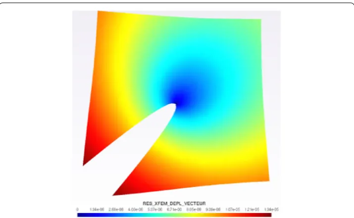
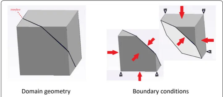
Example 1 (Horizontal crack opening in mode I with linear elements). The domain

geom-etry is a square defined by = [−0.5,+0.5]×[−0.5,+0.5].The meshing procedure subdivides the domain into regular sized cells, which edges are parallel to the crack. The size of the enrichment zone isr=0.1.

The analytical solution in displacement corresponds to the exact mode I limited to the

√

rterm in Williams series expansion [11] and is given by the first term of (15). Then, Dirichlet boundary conditions are applied on three sides. On the left side, Neumann conditions are preferred. As the left side is cut by the crack, Dirichlet conditions are more difficult to apply given the discontinuity of the displacement field (Fig.20).

The condition number is estimated by MUMPS solver, so that the results shown here have to be taken only as rough estimates.

On Fig.21, the condition number of X-FEM almost skyrockets as noticed in [21]. We did not consider the pre-conditioner of [21] here to show how both enrichment strategies, scalar and vectorial, behave without expensive treatment. Even the conditioning slope of the vectorial enrichment is far from optimal. The expected optimal conditioning slope is two [25].

Then, the relative error in energy norm is computed accordingly to the following for-mula:

u−uhenergy =

'$

σh_−σ:εh_−εd

,$

Fig. 19 Asymptotic behavior with Bernstein polynomials with dedicated pre-conditioners (same pre-conditioners as with linear elements). As with Lagrange polynomials, dedicated pre-conditioners do not solve accuracy issues

Fig. 20 Boundary conditions around the patch-test. Mixed boundary conditions are applied to avoid enforcing displacement on the nodes of the boundary near the crack interface which would add only a technical difficulty beyond the scope of the paper

On Fig.22, the rate of convergence in energy norm of the X-FEM scalar enrichment is under-optimal (around 0.91) as noticed in [17]. Optimality is recovered with the vectorial enrichment, the convergence rate being then 0.989. Nonetheless, X-FEM is more accurate than the vectorial enrichment as predicted in Lemma 1.

Example 2 (Inclined crack opening in mode I with linear elements). We introduce a more

Fig. 21 Conditioning of crack approximations. The condition number increases swiftly with the geometrical enrichment strategy i.e. the introduction of singular functions on many layers of elements around the crack-tip

Fig. 22 Convergence analysis of crack approximation spaces. The single-layer enrichment (topological) convergence curves are added to recall the benefit of the geometrical enrichment strategy

are applied (Fig.24), similarly to the case of the horizontal crack. We consider the same regular meshes as above which are not oriented accordingly to the crack surface here. The pre-conditioner of [21] is not applied here as in the previous case.

Fig. 23 Analytical solution corresponding to a mode 1 displacement field for the inclined crack

Fig. 24 Boundary conditions for an inclined crack. The boundary conditions are the same with the horizontal crack test

Fig. 26 Convergence analysis for vectorial and scalar enrichments with a crack orientation at 44.9◦. Both enrichments have optimal convergence order but error levels are quite high. Results are in accordance with the ones of Fig.22and X-FEM is more accurate than GFEM

Numerical analysis of crack approximation with quadratic elements: crack opening in mode 1 Only the linear vectorial enrichment approximation [30] is working with a reasonable condition number. We recall that other approximations are not tested because,

• X-FEM conditioning skyrockets with quadratic elements, even with a small enrich-ment zone,

• Gupta et al.SGFEM kind of enrichment [25,31] needs far too many additional

Heav-iside d.o.f., so that it is difficult to implement and may lead to ill conditioning,

• Cut-off with global d.o.f. assembling requires a “macro” element, which is not straight-forward to implement in finite element software. Moreover the method does not extend properly in 3D [29].

Even if the linear vectorial enrichment converges at an optimal rate (in energy norm) with quadratic elements, the condition number is still very high (see Fig.27). We did not use the pre-conditioner of [21], in order to test the conditioning of the vectorial enrichment. In “Singular approximation at a crack tip” section, a new enrichment strategy with better intrinsic numerical behavior, will be exposed.

Remark a dedicated integration scheme is needed at the tip of the crack, to get an optimal

rate of convergence in energy norm with quadratic elements [17]. Here, we used a Gauss-Radau integration rule of order 20 [39]. As the aim of the paper is not about singular integration, we did not try to optimize the procedure. Optimization of integration schemes has been well studied in [30,40].

Improving the design of quadratic approximation spaces to deal with previous numerical issues

In this section, basic improvements are suggested to deal with numerical issues stated in previous sections:

con-Fig. 27 Numerical behavior of the X-FEM vectorial enrichment with quadratic elements

vergence rates can only be achieved if the discontinuous approximation space is of the same order than the one of the continuous space, that is to say quadratic. The correction exposed here on the quadratic form is slightly different from the ones dis-cussed in “Strong discontinuity approximation conditioning” section (fit-to-vertex and elimination of d.o.f.).

– For singular enrichment, a reshape of the approximation space is considered. The new approximation sums up benefits of work on strong approximation spaces with the significant improvement associated to the “bubble” space as discussed in the next section.

Improvement of strongly discontinuous approximations Partition of unity alteration

As discussed in “Numerical analysis of strongly discontinuous approximations with quadratic elements” section, the use of vertex node and middle node shape functions (resp.χ+ΦSandχ+ΦMin Fig.16) leads to an incorrect asymptotic behavior of strongly discontinuous formulations, both for Bernstein and Lagrange polynomials.

When getting rid of the middle node d.o.f.χ+ΦM forεaround 10−3_{, the condition} number decreases sharply (Fig.28). This threshold value is close to estimates of [18,24], but we stress on the fact that only the middle d.o.f. is removed and that the position of the interface is not shifted. This alteration process allows the analysis to proceed beyond ε=10−12as with linear elements.

Let us precise the differences between the removal of the middle node and straightfor-ward criteria from “Strong discontinuity approximation conditioning” section:

• The fit-to-vertex and volume criterion remove both the vertex node and the middle node d.o.f. (χ+ΦSandχ₊ΦM). Then, with the fit-to-vertex, the interface position is switched to the closest node.

• With the new strategy, only the minimal information is removed from the approxima-tion (a single d.o.f., the nearest to the interface) with a tuned threshold. The interface is not switched.

Fig. 28 H1-error with quadratic Lagrange polynomials. The enrichments are alternated through the removal of the middle node beyond a threshold eps ofε=10−3

• The exact solution is continuous,

• In [7,26] discontinuous functions are added to continuous functions, so that the removal of the discontinuous middle node d.o.f. does not alter the partition of unity of continuous space functions [9] and consequently the representation of continuous functions.

This is in contrast with [33], as the removal of the enriched middle node d.o.f. prevents the representation of continuous functions on some parts of the domain where the partition of unity is broken.

Extrapolation in 3D

Let us consider the patch-test of [24]. It is a 3D block of side 4m defined by=[−2,+2]× [−2,+2]×[−2,+2] and split by an inclined interface. The domain is meshed with regular quadratic hexahedral elements (4 ×4 × 4 elements).

A multi-axial loading is applied. Given the elastic behavior, the stress is homogeneous within the block at a value of 10 MPa, for any given position of the interface. The interface equation is parameterized withδas:

x+y+z+δ=0 (51)

The error is analyzed with the energy norm:

u−uhenergy =

'$

σh_−σ:εh_−εd

,$

σ :εd (52)

As the Hansbo et al. [33] enrichment performs as well as the “shifted” enrichment, only the “shifted” enrichment is tested here.

The strategies discussed in 1D are extrapolated in 3D (an example is given Fig.29):

Fig. 29 3D test-case with quadratic elements. The strategies to improve the condition number are assessed on a 3D patch-test

• The elimination threshold for the middle nodes, is fixed at a ratio of relative distance to the vertex of 10−3along the edge (see on the 1D example illustrated by Fig.16), or, could be expressed with a volume ratio criterion [24]:

min

-measure(+∩Supp(ΦM)),

measure(−∩Supp(ΦM))

.

≤10−9measure(Supp(ΦM)) (53)

On (Fig.30), the shifted formulation is more accurate than the X-FEM one, as observed in the 1D case. The difference in accuracy reaches a 1010_{factor: accuracy issues observed} in 1D with X-FEM are heightened in 3D.

Furthermore, the volume ratio criterion on the middle node is very satisfactory. The results improve as soon as the elimination process is activated around a node to interface distance (hereδ/√3) of 10−3m.

Synthesis

Although, all three strongly discontinuous formulations considered in the paper represent the same approximation space, they do not have the same numerical performance. From the results above, domain and shifted enrichments are less sensitive to the position of the interface than X-FEM. With quadratic elements, the three formulations need a special care regarding the asymptotic behavior of the shape functions as shown in “Numerical

analysis of strongly discontinuous approximations with quadratic elements” section. The X-FEM jump formulation is far less accurate in 3D.

From a practical point of view, the “shifted” formulation seems to offer the best com-promise, because it provides:

• A simpler pre-conditioner than X-FEM, which decreases the computational cost, • Less discontinuous d.o.f. than [33], which eases the implementation and improves the

accuracy of the formulation in case of elimination of d.o.f. with Lagrange polynomials, • A good accuracy in 3D with quadratic elements.

Singular approximation at a crack tip

New “bubble” approximation space

We introduce a simpler space than the one of Gupta et al. [25,31], to reduce its too many additional Heaviside d.o.f. As a matter of fact Gupta et al. approach requires up to 12 Heaviside d.o.f. per node instead of 3 so that it is difficult to implement and may lead to ill conditioning.

In the elements where K_α is discontinuous, a technique similar to the ghost node interpolation used in [41] is preferred. The principle consists in using two continuous interpolations by prolongation of the one on₊and the one on₋to the whole domain (an example is given Fig.31). Hence, two continuous extensions ofK_α(r,θ) are introduced:

• K_α(r,|θ|) overlaps withK_α(r,θ) on₊, • K_α(r,− |θ|) overlaps withK_α(r,θ) on₋.

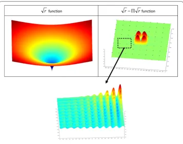
In the elements whereK_α has a singular point, the interpolation ofK_α is smoothened, so that subsequent interpolation errors of the singular function K_α do not pollute the accuracy of the displacement field as observed in [25].

Letnbe the order of the interpolation used for the crack tip degrees of freedom.ICTis the corresponding set of nodes enriched by the vectorial asymptotic functions i.e. ICT,1 corresponds to vertex nodes andICT,2contains both vertex nodes and middle nodes. If we consider a quadratic interpolation for the crack tip degrees of freedom, we haven=2 andICT,2=ICT. LetIT be the associated subset ofICTwith singular points i.e. the set of nodes such that a crack-tip belongs to their support. The nodes ofIT are not taken into account in the interpolation ofK_α, so that the interpolation ofK_α is smooth when the polar coordinatergoes to zero. Letmbe the order of the interpolation ofK_α, which can be different fromn. The new interpolation operator reads:

˜ m_K

α =

k∈{{ICT,m∪δICT,m}/IT}/IH

K_α(rk,θk)k,m

+

k∈IH∩{{ICT,m∪δICT,m}/IT}

K_α(r_k,|θk|)k,mχ++K_α(r_k,− |θk|)k,mχ− (54)

wherek,mare the shape functions corresponding to orderminterpolation andICT,mis the subset of ICT corresponding to order minterpolation, i.e. ICT,1is the restriction of ICT to vertex nodes andICT,2contains both vertex nodes and middle nodes of ICT. Since we consider quadratic approximation in this section, we haveICT,2=ICT. The set

ICT,m∪δICT,m

contains all the nodes lying in the support of a node ofICT.

This interpolation should be interpreted, for an element which is split by the interface (i.e. an element that does not contain a crack-tip), as follows

• Assuming the evaluation point (gauss point) is located on+, ˜

m_(K

α)=

k∈{ICT,m∪δICT,m}/IT

K_α(rk,|θk|)k,m (55)

• Assuming the evaluation point (gauss point) is located on₋, ˜

m_(K

α)=

k∈{ICT,m∪δICT,m}/IT

K_α(rk,− |θk|)k,m (56)

The new “bubble” approximation space, based on the new interpolation operator, is:

V_bub,m,nh =

⎧ ⎪ ⎪ ⎪ ⎨ ⎪ ⎪ ⎪ ⎩

vh=

i∈I d

j=1

ai,jΦiE_j+ i∈IH

d

j=1

bi,j(H−H(xi))ΦiEj

+

i∈ICT,n d

α=1

ci,αi,n

K_α−˜mK_α

⎫ ⎪ ⎪ ⎪ ⎬ ⎪ ⎪ ⎪ ⎭

(57)

whereΦiare the shape functions corresponding to the order of the elements, i.e. p=2 in this section andnrefers to the order of the shape functionsi,nused for the vectorial enrichment discretization.

Remark • Let us stress on the fact that the ghost node interpolation does not introduce

additional nodes. The two branches of discontinuous functions are interpolated over the element through extrapolation of branches (Fig.31);