R E S E A R C H
Open Access
The existence of equilibrium in a simple
exchange model
Piotr Ma´ckowiak
**Correspondence:
[email protected] Department of Mathematical Economics, Pozna ´n University of Economics, Al. Niepodległo´sci 10, Pozna ´n, 61-875, Poland
Abstract
This paper gives a new proof of the existence of equilibrium in a simple model of an exchange economy. We first formulate and prove a simple combinatorial lemma and then we use it to prove the existence of equilibrium. The combinatorial lemma allows us to derive an algorithm for the computation of equilibria. Though the existence theorem is formulated for functions defined on open simplices, it is equivalent to the Brouwer fixed point theorem.
MSC: Primary 91B02; secondary 91B50; 54H25
Keywords: simple exchange model; equilibrium existence; zero of a function; fixed point; computation of equilibria; simplicial methods
1 Introduction
Consider an economy withngoods populated with a finite numbermof consumers whose preferencesi, defined onRn
+, are continuous, strictly monotone and strictly convex.a
Suppose also that each consumer possesses a stockωi∈Rn+ of goods and that the (to-tal) supplyω=ω+· · ·+ωmis positive,ω> . Suppose that at each positive price vector
p= (p, . . . ,pn) each consumeriwants to maximize his/her preferences among affordable
bundles of goods,i.e., he/she plans to buy a bundle of goodsxi(p)∈Rnsuch that its value
pxi(p) is not greater than the valuepωi of the disposable stockωiandxi(p) is the best among affordable bundles:px≤pωi,x∈Rn+,x= xi(p) impliesxi(p)ixand it is not true thatxixi(p). The monotonicity of preferences implies thatpxi(p) =pωi. Hence, at the given pricesp, it holdspx(p) =pω, wherex(p) =x(p) +· · ·+xn(p) is the (total) demand for goods at pricesp. Plans of all consumers can come into effect only ifx(p) =ω- again by the monotonicity assumption on preferences. Does there exist an equilibrium price vec-tor,i.e., a positive price vectorpsuch thatx(p) =ω? It is well known that the answer to that question is positive; see [] for a survey of the basic existence results. It is obvious thatpis an equilibrium price vector if and only if the differencez(p) :=x(p) –ωvanishes. If we allowpto vary over the positive orthant ofRn, we obtain the functionz; the excess demand function of the economy. One can show thatzis homogeneous of degree zero, continuous on the set of positive prices, it satisfies Walras’ law and a boundary condition, and it is bounded from below [, Theorem ..]. One can also show that if a functionf
defined on the positive orthant ofRnpossesses the properties listed in the previous sen-tence, then there exists an economy whose excess demand functionzis different fromf
only on a neighborhood of the boundary ofRn
+inRnand the set of equilibrium prices
forz coincides with the set of zeros off []. In this work, we are going to use the ex-cess demand approach to prove the existence of equilibrium [, Section ]: we just impose conditions a function should possess to be the excess demand function of an economy and then we prove that there exists an equilibrium price vector.bThe novelty of our approach is that we are proving the existence of equilibrium (see the theorem in Section ) in a new and constructive way.cIt is important to emphasize that we do not rely on the Sperner
lemma [, p.] to prove the result. Instead of that, we introduce a combinatorial lemma (Lemma ) formulated for a special triangulation of a closed simplex only. The particular triangulation decreases generality of the lemma but is computationally advantageous [, p.].d
In the next section, we introduce notation. Section presents necessary notions from combinatorial topology and ends with the combinatorial lemma (Lemma ). In Section , we define the notions of excess demand function and equilibrium, and then we derive some properties of excess demand functions. Finally, we prove the existence theorem. Section contains an algorithm for computation of equilibria. In Section , we clarify some dif-ferences between the boundary condition we use (see Definition ()) and the standard boundary condition met in the literature. We also present a connection between fixed points of continuous functions and equilibria (zeros) of excess demand functions. At the end of Section , we pose a few open questions.
2 Notation
Let N denote the set of positive integers and for any n∈ N let Rn denote the n -dimensional Euclidean space, and [n] :={, . . . ,n}, [] :=∅. Moreover, ei is theith unit vector of the standard basis of Rn, where i∈[n]. In what follows, forn∈N the set n:={x∈Rn
+:
n
i=xi= }, whereR+is the set of nonnegative real numbers, is the
stan-dard (n– )-dimensional (closed) simplex andintn:={x∈n:xi> ,i∈[n]}is its (rel-ative) interior. For a setX⊂Rn,∂(X) denotes its boundary (or relative boundary of the closure ofXifXis convex). For vectorsx,y∈Rntheir scalar product isxy=n
i=xiyi. The Euclidean norm ofx∈Rnis denoted by|x|. For any setA,#Adenotes its cardinality.
3 Definitions, facts and a combinatorial lemma
We need some more or less standard definitions and facts from combinatorial topology; they can be found in [] and []. Let us fixn∈N.
- Letvj∈Rn,j∈[k],k≤n+ , be affinely independent. The setσ defined as σ:={x∈Rn:x=k
j=αjvj,α∈k}is called a(k– )-simplex with verticesvj,j∈[k]. We write it briefly asσ=vj:j∈[k] orσ=v, . . . ,vk . If we know thatσ is a
(k– )-simplex, then the set of its vertices is denoted byV(σ). Ifp∈σ, then the vector αp:= (αp
, . . . ,α
p
k)∈kis called the vector of the barycentric coordinates ofpinσ, if
p=kj=αpjvj. For eachp∈σ, its barycentric coordinatesαpin the simplexσ are uniquely determined.
- Ifσis a(k– )-simplex, thenA , where∅ =A⊂V(σ), is called a(#A– )-face ofσ. - A collection{σj:j∈[J]},J∈N, of nonempty subsets of a(k– )-simplexS⊂Rn,
<k≤n+ , is called a triangulation ofSif it meets the following conditions: . σjis a(k– )-simplex,j∈[J],
- Two different(k– )-simplicesσj,σj,j,j∈[J],j=j, in a triangulation of a
(k– )-simplexSare adjacent ifV(σ)∩V(σ) is a(k– )-face for both of them. Each (k– )-face of a simplexσj,j∈[J], is a(k– )-face for exactly two different simplices in the triangulation, provided the(k– )-face is not contained in∂(S).
- TheK-triangulation of an(n– )-simplexS=v, . . . ,vn ⊂Rnwith grid sizem–,
wheremis a positive integer,eis the collection of all(n– )-simplicesσof the form
σ=p,p, . . . ,pn , where verticesp,p, . . . ,pn∈Ssatisfy the following conditions: . each barycentric coordinateαip,i∈[n], ofpinSis a nonnegative multiple
ofm–,
. αpj+=αpj+m–(eπj–eπj+), whereπ= (π
, . . . ,πn–)is a permutation of[n– ],
αplis the vector of the barycentric coordinates ofpl,l∈ {j,j+ },j∈[n– ]. TheK-triangulation ofSwith grid sizem–is denoted byK(S,m)and the set of all
vertices of simplices inK(S,m)is denoted byV(S,m). Obviously,
V(S,m) =σ∈K(S,m)V(σ) ={αv+· · ·+αnvn:α∈n,αi∈ {, /m, . . . , – /m, }}. For anyε> and for a sufficiently largem, each simplex inK(S,m)has the diameter not greater thanε. Moreover, there exists exactly one simplex inK(S,m)such thatvn is its vertex.f
A basic tool used in the proof of our main result is the following.
Lemma Let S:=v, . . . ,vn ⊂Rnbe an(n– )-simplex and l:V(S,m)→ {, , . . . ,n},
m≥,be a function satisfying for all p∈V(S,m)the following conditions: . αip= ⇒l(p)=i,i∈[n– ],
. l(p) = ifαpn= , . l(p) =nifαnp= ,
. l(p)∈[n– ]if <αpn< .
Then there exists a unique finite sequence of simplicesσ, . . . ,σJ∈K(S,m),J∈N,such that σjandσj+are adjacent for j∈[J– ],n∈l(σ), ∈l(σJ), [n– ]⊂l(σj),j∈[J],andσj+∈/
{σ, . . . ,σj},j∈[J– ].g
Proof Letσdenote the unique simplex inK(S,m) whose vertex ispn:=vn. Vectors of the
barycentric coordinates of vertices ofσ(other thanpn) are of the form
αpj=, . . . , , m–
jth coordinate
, , . . . , , –m– , j∈[n– ].
Sinceαipj = impliesl(pj)=i, thenl(pj) =j,j∈[n] and therefore [n– ]⊂l(σ
).
More-over, since for allv∈V(S,m)αv
i = impliesl(v)=i, thenl(σ) = [n– ] entailsσis not contained in∂(S), whereσis an (n– )-face of someσ∈K(S,m). Whence, no (n– )-face ofσ∈K(S,m) on whose vertices functionlassumes all values in [n– ] is contained in the boundary ofS. Further, there exists exactly oneσ∈K(S,m)\{σ}, which is
adja-cent toσ. Obviously,l(σ) = [n– ]. Letpn+ be the only element ofV(σ)\V(σ). Since l({p, . . . ,pn–}) = [n– ] andl(pn+)∈[n– ], there exists exactly one vertexpi among p, . . . ,pn–such thatl(pi) =l(pn+) and functionlattains all values in [n– ] on the (n–
)-face V(σ)\{pi} . So, we can find a simplexσ
∈K(S,m)\{σ,σ}adjacent toσ with
[n– ]⊂l(σ), and if ∈l(σ) - the process is complete, if not - proceeding as earlier
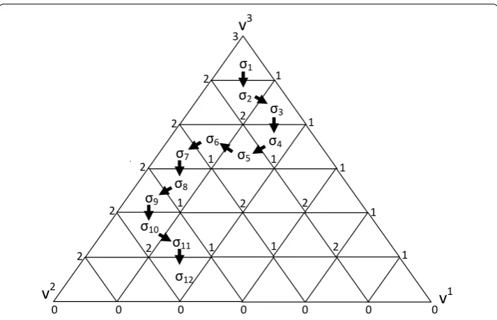
Figure 1 TheK-triangulation of 2-simplexS=v1,v2,v3with grid size 6. The small triangles are members of the triangulationK(S, 6). The number at a vertex of a simplex inK(S, 6) is the value oflassigned to the vertex and one sees thatlsatisfies the assumptions of Lemma 1. The sequence of simplicesσ1,. . .,σ12
meets the requirements described in the proof of Lemma 1.
the sequenceσ, . . . ,σJ. If ∈l(σJ), then the sequence satisfies the claim. Suppose that /∈l(σJ). Since each (n– )-face which is not contained in∂(S) is shared by exactly two simplices ofK(S,m), there exists precisely one simplexσinK(S,m)\{σ, . . . ,σJ}such that σJandσshare the (n– )-faceσ∩σJwithl(σ∩σJ) = [n– ] - this ensures thatσJ+=σ
and that no simplex ofK(S,m) appears twice (or more) in the sequenceσ, . . . ,σJ+, where
/∈l(σJ). Thus, in view of the finiteness ofK(S,m) and sincel(σ) = [n– ] impliesσis not contained in∂(S), we conclude that there existsJ such that ∈l(σJ), otherwise we could construct an infinite sequence of simplices built of finitely many different elements ofK(S,m), which would imply that a simplex appears more than once in the sequence -which is an absurd. The choice ofσj+guarantees thatσj+∈ {/ σ, . . . ,σj},j∈[J– ]. Unique-ness of the constructed sequence comes from the preceding sentence, uniqueUnique-ness of the simplex containingvn, and the fact that each (n– )-face in the (relative) interior ofSis shared by exactly two simplices of the triangulation.
4 The existence of equilibrium
Definition Let us fixn∈N. We say that a functionz:intn→Rn,z(p) = (z(p), . . . , zn(p)), is an excess demand function, if it satisfies the following conditions:
. zis continuous onintn,
. Walras’ law holds, that is,pz(p) = forp∈intn,
. the boundary condition holds: ifpj∈intn,j∈N,limj→+∞pj=p∈∂(n)and pi= ,i∈[n], thenlimj→+∞zi(pj) = +∞,
. zis bounded from below:infp∈intnzi(p) > –∞,i∈[n].
The main goal of the paper is to give a new proof of the fact that for each excess demand function there exists an equilibrium point. First, we are going to characterize the behavior ofznear the (relative) boundary of its domain, which is crucial for the theorem to follow. The intuition for the lemma below is as follows: if the pricepiof a goodiis low (in com-parison to some other price - prices are standardized; they sum up to ) then the demand significantly exceeds the supply of that good; if the pricepiis (relatively) high - so all the other prices are low - then the demand for theith good is considerably less than its supply.
Lemma Let z:intn→Rnbe an excess demand function.Then there existsε
> such that for i∈[n]and p∈intnwe have
pi≤ε⇒zi(p) > and
pi≥ –ε⇒zi(p) < .
Proof Suppose that the former implication is not true. Then there existi∈[n] and a se-quencepj∈intn,j∈N:lim
j→+∞pj=p,pi= , andlimj→+∞zi(pj)≤ , which contradicts the boundary condition. This implies that there existsε> for which the just considered
implication is true and without loss of generality we can assume thatε< –ε. To prove
the latter implication, observe thatpi≥ –εimpliespi≤ε,i=i, so the first implication
guarantees thatzi(p) > ,i=i. Now, from Walras’ law, we get <
i=ipizi(p) = –pizi(p),
andzi(p) < is satisfied.
Lemma Let z andεbe as in Lemma.Let S:={p∈intn:pn∈(, –ε/]}and define
the functionz:intn→Rn–as follows: ∀p∈intn z(p) :=( –pn)zi(p) +pnzn(p)
n–
i=. ()
Then
. zis continuous,
. zis bounded from below:infp∈intnzi(p) > –∞,i∈[n– ],
. pz(p) +· · ·+pn–zn–(p) = forp∈intn,
. ifpj∈S
,j∈N,limj→+∞pj=p∈∂(n)andpi= ,i∈[n– ],then
limj→+∞zi(pj) = +∞,
. ∃ε∈(,ε/]∀p∈S∀i∈[n– ]:
pi≤ε⇒zi(p) > and
pi≥ –ε⇒zi(p) < .
Proof The continuity ofzis obvious. The boundedness from below ofzstems from the fact thatzis bounded from below and the weightspn, –pn, are positive and less than for allpn∈(, ). The following equalities show that property () is met:
pz(p) +· · ·+pn–zn–(p)
=p
( –pn)z(p) +pnzn(p) +· · ·+pn–
( –pn)zn–(p) +pnzn(p)
= ( –pn)pz(p) +· · ·+pn–zn–(p) + (p+· · ·+pn–) =–pn
pnzn(p)
If pj ∈S
, j∈N, converges to a point p with pi= for some i∈ [n– ] then ( –
pjn)zi(pj) diverges to +∞and since the productpjnzn(pj) is bounded from below it holds:
limj→+∞zi(pj) = +∞. To prove that () is true it suffices to observe that forp∈Swe have
–pn≥ε/ and to proceed as in the proof of Lemma withzin place ofz.
The formula used to define the functionzresembles the linear homotopy between func-tions
( –ε/)z(·,ε/) + (ε/)zn(·,ε/)n –
i=,
and
(ε/)z(·, –ε/) + ( –ε/)zn(·, –ε/) ni=–;
just puttin place ofpn, assume thattchanges fromε/ through –ε/ and the
‘homo-topy’ is
H(p, . . . ,pn–,t) :=
( –t)zi(·,t) +tzn(·,t) ni=–.
ButHis not a homotopy since the domain ofH(·,t) changes astchanges.
The important thing which Lemma reveals is that at each fixedpn∈(, ) the function
z(·,pn) is an excess demand function defined on a simplex of dimensionn– instead of
n– .i
Now suppose thatεandεsatisfy the statement of Lemma and let fori∈[n]:
ei:=
ε n– , . . . ,
ε
n– , – ε ith coordinate
, ε
n– , . . . , ε n–
∈intn. ()
We can assume that the vectorsei, i∈[n], are linearly independent; it suffices to take sufficiently smallε> . The setS:=ei:i∈[n] ⊂intnis an (n– )-simplex with the
verticesei,i∈[n]. Ifp∈S∩S, thenpi∈[ε/(n– ), –ε],i∈[n– ] and ifαip= (i.e.,
pi=ε/(n– ) <ε/) thenzi(p) > ; similarly, ifαip= (i.e. pi= –ε> –ε/) then
zi(p) < . Moreover, ifp∈Sandpn≥ –εthenzn(p) < and ifpn≤ε thenzn(p) >
(see Lemma ). We are now in a position to prove the main result of the paper.
Theorem Let z be as in Lemma.For eachε> there exists p∈intn:zi(p)≤ε,i∈[n].
Proof Ifn= , then there is nothing to prove:int={} ⊂R, and by Walras’ law,z(p) = at p= . Suppose thatn≥. Let us fixε> and define ε:=εε, whereε comes from
Lemma . Let alsoSbe as in the hypothesis of Lemma and letSbe the (n– )-simplex
with vertices given by (). By the continuity of the restriction ofzto the compact setS,
there existsδ> such that ifp,p∈Sand|p–p|<δ, then|z(p) –z(p)|<ε. Choose an
integerm≥ for which all simplices inK(S,m) have diameter less thanmin{δ,ε/}. Let kdenote the smallest integer in [m] for which ( –km)nε– + ( –ε)km≥ –ε- this ensures
satisfiespn≥–ε/. To justify this statement, observe that –ε–nε–≥–ε≥–ε>
andαnp≥k/mentail
pn=
–αpn ε
n– + ( –ε)α p n=
ε n– +
–ε–
ε n–
αpn
≥ ε n– +
–ε–
ε n–
k m=
–k
m
ε
n– + ( –ε)
k m
≥ –ε/.
The minimality ofkassures that for any nonnegative integerk<kifp∈Sandαpn≤k/m, thenpn< –ε/ andp∈S; the latter implies that the claim of Lemma () applies to p. Notice that ifp∈S andpn≥ –ε/ then zn(p) < and ifpn<ε/ then zn(p) > (see Lemma ). Let us define a functionlfrom the set of verticesV(S,m) to [n]∪ {}as
follows:j
l(p) =
⎧ ⎪ ⎪ ⎪ ⎪ ⎪ ⎨ ⎪ ⎪ ⎪ ⎪ ⎪ ⎩
n, ifαpn= ,
, ifαpn= ,
min{i∈[n– ] :αip> }, if >αnp≥k/m,
min{i∈[n– ] :zi(p)≤}, ifk/m>αnp> ,
()
wherezis defined in (). Fori∈[n– ], ifp∈V(S,m), >αnp≥k/m, andαip= then it is clear thatl(p)=i, since ifl(p) =i, then we would obtainαip> . Assume thatp∈V(S,m)
and <αnp<k/m. Sincep∈intn, Lemma () ensures thatzi(p)≤ for somei∈[n– ] - so,l(p) is well defined. Moreover,αpn<k/mimpliesαpn=k/mfor some nonnegative in-tegerksuch thatk<kand, therefore, due to Lemma (), it holds thatzi(p) > forαip= from which we obtainl(p)=iwheneverαpi = . Therefore, the assumptions of the com-binatorial Lemma are satisfied. Hence, there exists a sequence of simplicesσ, . . . ,σJ in K(S,m) such thatσjandσj+are adjacent andn∈l(σ), ∈l(σJ), [n– ]⊂l(σj),j∈[J]. There exists the first simplex in that sequence, call itσj, such that for allj>jthe last
barycentric coordinate of all vertices ofσjinS are less thank/m. Simplicesσj∩σj+
are adjacent,i.e.they share an (n– )-face, and in other words, they differ by one ver-tex only. By the choice ofj all verticesp∈V(σj+) satisfyαnp<k/m, and there is a
ver-texp∈V(σj)\V(σj+) such thatα
p
n≥k/m. Now, the adjacency ofσjandσj+, the fact
that all simplices inK(S,m) have diameters less thanε/ and the inequalitypn≥ –ε/
entail thatpn≥ –ε forp∈V(σj+), which implieszn(p) < forp∈V(σj+).
Reason-ing analogously, we get for the last simplex,σJ, that it holds:zn(p) > ,p∈V(σJ). By the choice ofj, all simplicesσj,j≥j+ , are contained inS∩S. Moreover, their
diame-ters are less thanδ so p,p∈σj,j≥j+ , implies|zi(p) –zi(p)| ≤ε, i∈[n– ]. Since
j≥jσjis (arcwise) connected andV(σj)∩zn–((–∞, ))=∅andV(σJ)∩zn–((, +∞))=∅ then by the continuity ofzthere exists a simplexσj,j≥j+ : ∈zn(σj). Letp∈σj : zn(p) = . So|p–p|<δ,p∈V(σj). Since for eachi, there exists a vertexpiofσj such
thatzi(pi)≤ (by the inclusion [n– ]⊂l(σj)), ( –pn)zi(p) =zi(p)≤zi(p
i) +ε≤ε,
i∈[n– ]. Further,zi(p)≤ (–εp
n) ≤
ε
ε =ε,i∈[n– ], sincepn∈[ε, –ε], ifzn(p) = ,
due to Lemma . We have found a point p∈intn:zi(p)≤ε, i∈[n], which ends the
Figure 2 This figure explains the idea of the proof of theorem forn= 3. Values oflassigned to the vertices inV(S2,m) are independent ofzif the considered vertex is above or on the linep3≤1 –ε1/2 - here
the second and third row of the formula (3) are used to define vales ofl. If a vertex is below the line
p3≤1 –ε1/2 - but not at the bottom ofS2- thenzis used to compute the value ofl. The thick curve presents
a hypothetical sequence of simplicesσ1,. . .,σJ. For vertices of simplices above (p3≥1 –ε1)-line (below
(p3≤ε1)-line) values ofznare negative (positive). Ifσjis below (p3≤1 –ε1/2)-line then each coordinate ofz
admits a non-positive value at a vertex ofσj. Somewhere between (p3≥1 –ε1) and (p3≤ε1)-lines there is a
simplexσjsuch thatzn(p)zn(p)≤0 for a pair of verticesp,pofσj- that simplex is what we are looking for.
Figure illustrates the proof.
Corollary Let z be as in the above theorem.There exists an equilibrium point for z.
Proof Letεq> ,q∈N, be a sequence converging to . In view of the proof of the theorem, for eachq∈Nthere exists a pointpq∈S
such thatzi(pq)≤εq, i∈[n]. The Bolzano-Weierstrass theorem and compactness ofS imply that there exists a convergent
sub-sequence pq ofpq, such thatlim
q→+∞pq
=p∈S. From the continuity of z, it follows
thatzi(p)≤, fori∈[n]. Sincep∈S⊂intn,pi> ,i∈[n]. Walras’ law ensures that
z(p) = .
5 An algorithm for the computation of equilibrium
From the proof of the theorem, we can derive the following algorithm for computation of a point p∈intnsatisfyingzi(p)≤ε,i∈[n], whereε> is a given accuracy level. The algorithm below uses the functionl:V(S,m)→ {, , . . . ,n}defined in () and we
reasonably assume thatn≥.
Step 0: Determineε,εsatisfying claim of Lemma 2 and Lemma 3(5),
respectively. Fix accuracy level:ε> .Findδ> such that
ifp,p∈S, where S is defined as in the proof of the
integer for which all simplices inK(S,m) have diameter
less thanmin{δ,ε/}.Let σ be is as in the proof of Lemma 1
forS=S, setFaceVertices:=V(σ)\{en},v:=en(see formula (2))
and go to step 1.
Step 1: Determine the only vertex v ∈ V(S,m) such that v = v and
FaceVertices∪ {v} ∈K(S,m). Go to step 2.
Step 2: IfFaceVertices∪ {v} ⊂S, where S is defined in Lemma 3, and
zn(v) > STOP: v satisfies zi(v) ≤ ε, i ∈ [n]. Otherwise,
assign the only element ofl–(l(v))∩FaceVerticesas the value ofv.
SetFaceVertices:= (FaceVertices\{v})∪ {v}and go to step 1.
Step initializes the necessary parameters for correct course of the algorithm and in fact it is the most difficult part of the algorithm, unless we know some properties of the con-sidered excess demand function (e.g., differentiability, its lower bound or if it is a Lip-schitz function on compact subsets of intn). It is easy to determinemif we know δ andε; it suffices to takem≥ (n–)
√
min{δ,ε/}, which is a consequence of the definition of the K-triangulation and the fact that the diameter of a simplex equals the maximum dis-tance between its vertices. In Steps and , set FaceVertices is a face of an element of K(S,m) such thatl(FaceVertices) = [n– ]. In Step , we check if currently
consid-ered simplexFaceVertices∪ {v} , wherevis such a vertex inK(S,m) thatFaceVertices
is common (n– )-face of the currently considered simplex and its direct predecessor FaceVertices∪ {v} , is contained inS, which implies that the value ofldepends on
func-tionz(see Lemma and formula ()). If it is the case, and in additionzn(v) > , thenvis what we seek for. If not, we have to find the next adjacent simplex; to this goal, we have to decide which vertex should be removed fromFaceVertices. To achieve this, we find the vertexv∈FaceVertices, which bears the same value ofl asvand we form the new set
FaceVerticessubstitutingvin place ofvand then we repeat the operations. The algorithm succeeds in finding approximate zero in a finite number of iterations due to Lemma , the theorem and its proof. It is worth to emphasize that at a given iteration of the algorithm (Step -Step ) exactly one new value oflis computed and to proceed on with computa-tions it is sufficient to know only the last simplex; there is no need to remember the earlier stages in the course of the algorithm. Moreover, the values oflneed to be computed only at the vertices of the constructed sequence of simplices.
6 Final comments
6.1 The boundary condition
The standard form of the boundary condition imposed on/satisfied by an excess demand functions is:kpj∈intn,j∈N,lim
j→+∞pj=p∈∂(n),pi= , implieslimj→+∞max{zi(pj) :
6.2 Fixed points of continuous functions defined on the standard simplex
Here, we show how to relate a continuous functionf :n→nand an excess demand function, for which we can apply our algorithm and we can find approximate fixed points off. We use a construction by Uzawa []. Let a continuous functiong:n→Rnbe defined as
∀x∈n:g(x) :=f(x) –xf(x)
xx x.
Sincexg(x) =xf(x) –xf(x) = , then the functiongmeets Walras’ law. Let us fix a number
h> and define a functionzh:intn→Rnas
zh(x) =zh(x), . . . ,znh(x) :=g(x) +h
(nx)–– , . . . ,gn(x) +h
(nxn)–– .
One can easily check thatzhis an excess demand function. Now, by the corollary, we see that for eachh> there exists a pointxh∈intn:zh(xh) = , written equivalently as
gi
xh = –h
nxhi –
, i∈[n].
Leth→+andxh→x∈n(taking a subsequence if necessary). Ifx
i> , thengi(x) = . If xi= then nxh
i →
+∞and
nxhi – →+∞, so –h(
nxhi – ) < , but boundedness ofg implies that –h(
nxh i
– ),h> , is bounded. We obtaing(x)≤, which ensures thatf(x) =x
(see []). Hence, to find an approximate fixed point off, we can apply the algorithm for
zh,hsufficiently small.
The equivalence of the existence of equilibria for excess demand functions defined on the standard closed simplicesland Brouwer’s theorem was shown in []. The proofs of the
equivalence for the excess demand functions considered in the current paper can be found in [] or [].
6.3 Open questions
Combinatorial Lemma seems to be interesting for its own sake in spite of the fact that it is proved for a particular triangulation. We have seen that it implies the existence of equi-librium for an excess demand function. A slight modification of the proof of Theorem in [] allows to claim that the existence of equilibrium for an excess demand function is equivalent to the Brouwer fixed point theorem (see also []). The famous Sperner lemma, which is a combinatorial tool used to prove Brouwer’s fixed point theorem (and which is equivalent to it [, p.]) has many implications (e.g., see [, pp.-]). What are other implications of Lemma ? Does Lemma generalize to any triangulation of the standard simplex? Is it equivalent to Sperner’s lemma? What about the behavior of the algorithm presented in the paper in comparison to the behavior of other computational methods for finding equilibria (e.g., methods presented in [])? How to modify the algorithm to allow for the computation of (approximate) equilibria of excess demand mappings rather than functions?
Competing interests
Acknowledgements
I would like to thank participants of the Seminar of Department of Mathematical Economics (Pozna ´n University of Economics), Nonlinear Analysis Seminar at Faculty of Mathematics and Computer Science (Adam Mickiewicz University in Pozna ´n), Seminar of the Game and Decision Theory at Institute of Computer Science (Polish Academy of Science, Warsaw) for helpful comments and criticism. I also thank the referees for their comments and remarks that improved the paper. All remaining errors are mine. This work was financially supported by the Polish National Science Centre, grant no. UMO-2011/01/B/HS4/02219.
Endnotes
a Precise definitions can be found in [1] or [2, Chapter 1]. The presented description of exchange economies goes along the lines of [2, pp.29-31] and is rather standard.
b Homogeneity of degree zero is among these conditions: we can restrict our considerations to excess demand functions defined on the open standard simplex and not on the whole positive orthant ofRn- see Definition 1 in
Section 4.
c Constructivein the sense that it allows to derive a (simplicial) algorithm for computation of an approximate equilibrium.
d We find [4] by Yang as a comprehensive source of information on computation of equilibria and fixed points. Since the primary goal of this paper is to derive the existence of equilibria in a novel way without referring to Brouwer’s fixed point theorem and not to construct algorithm for computation of equilibria, the algorithm presented below should be treated as a by-product which is important, as we believe, but whose properties should be examined in the future.
e OurK-triangulation is called theK
2(m)-triangulation in [4, p.64].
f We could not have found a reference for this statement but it is proof is elementary.
g For simplicity: if we know thatσis a simplex we writel(σ) instead of - formally correct way -l(V(σ)). Notice, that the codomain of the functionlcould be easily changed to [n– 1] in place of [n]∪ {0}, but we do not do that to discern the ’top’ of a simplex from its ’bottom’ - see Figure 1.
h The method of construction of the sequence is similar to the one used in the proof of the correctness of the Scarf algorithm - see [4, p.68].
i The idea for the definition ofzcomes from the proof of Theorem 1 in [6] as it comes as a loose suggestion for the proof of our main theorem below.
j The idea forlis closely related to the notion of the standard integer labeling rule [4, p.63]. k See [2, Theorem 1.4.4] or [1, Lemma 4].
l This assumption eliminates both boundary conditions presented above.
Received: 11 January 2013 Accepted: 5 April 2013 Published: 18 April 2013 References
1. Debreu, G: Existence of competitive equilibrium. In: Arrow, KJ, Intriligator, MD (eds.) Handbook of Mathematical Economics, vol. 2, pp. 697-743. North-Holland, Amsterdam (1982)
2. Aliprantis, C, Brown, D, Burkinshaw, O: Existence and Optimality of Competitive Equilibria. Springer, Berlin (1990) 3. Mas-Colell, A: On the equilibrium price set of an exchange economy. J. Math. Econ.4, 117-126 (1977) 4. Yang, Z: Computing Equilibria and Fixed Points. Kluwer, Boston (1999)
5. Scarf, H: The computation of equilibrium prices: an exposition. In: Arrow, KJ, Intriligator, MD (eds.) Handbook of Mathematical Economics, vol. 2, pp. 1006-1061. North-Holland, Amsterdam (1982)
6. Ma´ckowiak, P: The existence of equilibrium without fixed-point arguments. J. Math. Econ.46(6), 1194-1199 (2010) 7. Uzawa, H: Walras’ existence theorem and Brouwer’s fixed-point theorem. Econ. Stud. Q.13(1), 59-62 (1962) 8. Ma´ckowiak, P: Some equivalents of Brouwer’s fixed point theorem and the existence of economic equilibrium. In:
Matłoka, M (ed.) Quantitative Methods in Economics. Scientific Books, vol. 222, pp. 164-171. Pozna ´n University of Economics Press, Pozna ´n (2012)
9. Toda, M: Approximation of excess demand on the boundary and equilibrium price set. Adv. Math. Econ.9, 99-107 (2006)
10. Dugundji, J, Granas, A: Fixed Point Theory. Springer, New York (2003)
doi:10.1186/1687-1812-2013-104