R E S E A R C H
Open Access
Speaker adaptation based on regularized
speaker-dependent eigenphone matrix
estimation
Wen-Lin Zhang
1*, Wei-Qiang Zhang
2, Dan Qu
1and Bi-Cheng Li
1Abstract
Eigenphone-based speaker adaptation outperforms conventional maximum likelihood linear regression (MLLR) and eigenvoice methods when there is sufficient adaptation data. However, it suffers from severe over-fitting when only a few seconds of adaptation data are provided. In this paper, various regularization methods are investigated to obtain a more robust speaker-dependent eigenphone matrix estimation. Element-wisel1norm regularization (known as
lasso) encourages the eigenphone matrix to be sparse, which reduces the number of effective free parameters and improves generalization. Squaredl2norm regularization promotes an element-wise shrinkage of the estimated matrix
towards zero, thus alleviating over-fitting. Column-wise unsquaredl2norm regularization (known as group lasso) acts
like the lasso at the column level, encouraging column sparsity in the eigenphone matrix, i.e., preferring an
eigenphone matrix with many zero columns as solution. Each column corresponds to an eigenphone, which is a basis vector of the phone variation subspace. Thus, group lasso tries to prevent the dimensionality of the subspace from growing beyond what is necessary. For nonzero columns, group lasso acts like a squaredl2norm regularization with
an adaptive weighting factor at the column level. Two combinations of these methods are also investigated, namely elastic net (applyingl1and squaredl2norms simultaneously) and sparse group lasso (applyingl1and column-wise
unsquaredl2norms simultaneously). Furthermore, a simplified method for estimating the eigenphone matrix in case
of diagonal covariance matrices is derived, and a unified framework for solving various regularized matrix estimation problems is presented. Experimental results show that these methods improve the adaptation performance
substantially, especially when the amount of adaptation data is limited. The best results are obtained when using the sparse group lasso method, which combines the advantages of both the lasso and group lasso methods. Using speaker-adaptive training, performance can be further improved.
Keywords: Eigenphones; Speaker adaptation; Regularization methods; Sparse group lasso
1 Introduction
Model space speaker adaptation is an important tech-nique in modern speech recognition system. The basic idea is that given some adaptation data, the parameters of a speaker-independent (SI) system are transformed to match the speaking pattern of an unknown speaker, result-ing in a speaker-adapted (SA) system. In this paper, we focus on the speaker adaptation of a conventional hidden Markov model Gaussian mixture model (HMM-GMM)-based speech recognition system. To deal with the scarcity
*Correspondence: [email protected]
1Zhengzhou Information Science and Technology Institute, Zhengzhou 450000, China
Full list of author information is available at the end of the article
of the adaptation data, parameter sharing schemes are usually adopted. For example, in the eigenvoice method [1], the SA models are assumed to lie in a low-dimensional speaker subspace. The subspace bases are shared among all speakers, and a speaker dependent coordinate vector is estimated for each unknown speaker. The maximum likelihood linear regression (MLLR) method [2] estimates a set of linear transformations to transform an SI model into an SA model. The transformation matrices are shared among different HMM state components.
Recently, a novel phone subspace-based method, the eigenphone-based method, was proposed [3]. In con-trast to the eigenvoice method, the phone variations of a speaker are assumed to be in a low-dimensional subspace,
called the phone variation subspace. The coordinates of the whole phone set are shared among different speakers. During speaker adaptation, a speaker-dependent eigen-phone matrix representing the main eigen-phone variation patterns for a specific speaker is estimated. In [4], the ‘eigenphone’ is first introduced as a set of linear basis vectors of the phone space used in conjunction with eigen-voices. The set of linear basis vectors are obtained by a Kullback-Leibler divergence minimization algorithm for a closed set of training speakers. Estimation of the eigen-phones for unknown speakers is not studied. Kenny’s eigenphone method is a multi-speaker modeling tech-nique rather than a speaker adaptation techtech-nique in the usual sense. In our method, the speaker-independent phone coordinate matrix is obtained by principal compo-nent analysis (PCA), and speaker adaptation is performed by estimating a set of eigenphones for each unknown speaker using the maximum likelihood criterion.
Due to its more elaborate modeling, the eigenphone method outperforms both the eigenvoice and the MLLR method, when sufficient amounts of adaptation data are available. However, with limited amounts of adaptation data, the estimation shows severe over-fitting, resulting in very bad adaptation performance [3]. Even with a fine tuned Gaussian prior, the eigenphone matrix estimated by the maximuma posteriori(MAP) criterion still does not match the performance of the eigenvoice method.
In machine learning, regularization techniques are widely employed to address the problem of data scarcity and model complexity. Recently, regularization has been widely adopted in speech processing and speech recog-nition applications. For instance,l1andl2regularization
have been proposed for spectral denoising in speech recognition [5]. In [6], similar regularization methods are adopted to improve the estimation of state-specific parameters in the subspace Gaussian mixture model (SGMM). In [7],l1 regularization is used to reduce the
nonzero connections of deep neural networks (DNNs) without sacrificing speech recognition performance. In [8], it was found that group sparse regularization can offer significant gains over efficient techniques like the elastic net (combining ofl1andl2regularization) in noise robust
speech recognition.
In this paper, we investigate the regularized estimation of the speaker-dependent eigenphone matrix for speaker adaptation. Three regularization methods and their com-binations are applied to improve the robustness of the
eigenphone-based method. The l1 norm regularization
can be used to constrain the sparsity of the matrix, which can reduce the number of free parameters of each eigenphone, thus improving the robustness of the adapta-tion. The squaredl2norm can prevent each eigenphone
from being too large, yielding better generalization of the adapted model. Each column in the eigenphone matrix
corresponds to one eigenphone and hence is a basis vec-tor of the phone variation subspace. Thus, the number of nonzero columns determines the dimension of the phone variation subspace. The column-wise unsquaredl2norm
regularization forces some columns of the matrix to be zero, thus effectively preventing the dimensionality of the phone variation subspace to grow beyond what is neces-sary. In this paper, all these regularization methods, as well as two combinations of them, namely, the elastic net and sparse group lasso, are presented in a unified framework. Accelerated proximal gradient descent is adopted to solve the mathematical optimization problems in a flexible way. In [9], a speaker-space compressive sensing method is used to perform speaker adaptation using an over-complete speaker dictionary in case of limited amount of adaptation data. In this paper, we discuss the phone-space speaker adaptation method, which obtains good perfor-mance when the adaptation data is sufficient. Various regularization methods are applied to improve perfor-mance in case of insufficient adaptation data. Although the speaker-space and phone-space methods can be com-bined using a hierarchical Bayesian framework [10], we will not pursue that in this paper.
In the next section, a brief overview of the eigenphone-based speaker adaptation method is given, a simplified method for row-wise estimation of the eigenphone matrix in case of diagonal covariance matrices is derived, and the comparisons between the eigenphone method and various existing methods are presented. A unified frame-work of regularized eigenphone estimation is proposed in Section 3. Various regularization methods and their com-binations are discussed in detail. The optimization of the eigenphone matrix using an accelerated incremental prox-imal gradient decent algorithm is given in Section 4. In Section 5, different regularization methods are compared through experiments on supervised speaker adaptation of a Mandarin syllable recognition system and unsupervised speaker adaptation of an English large vocabulary speech recognition system using the Wall Street Journal (WSJ; New York, NY, USA) corpus. Finally, conclusions are given in Section 6.
2 Review of the eigenphone-based speaker adaptation method
2.1 Eigenphone-based speaker adaptation
Given a set of speaker-independent HMMs containing a total ofMmixture components across all states and mod-els and a D-dimensional speech feature vector, let μm, μm(s), andum(s)=μm(s)−μmdenote the SI mean vec-tor, the SA mean vecvec-tor, and the phone variation vector for speakersand mixture componentm, respectively. In eigenphone-based speaker adaptation method, the phone variation vectors {um(s)}Mm=1 are assumed to be located
variation subspace. The eigenphone decomposition of the phone variation matrix can be expressed by the following equation [3]:
U(s)=[u1(s)u2(s)· · ·uM(s)]
≈[v0(s)v1(s)v2(s)· · ·vN(s)] ⎡ ⎢ ⎢ ⎢ ⎢ ⎢ ⎣
1 1 1 . . . 1 l11 l21 l31 . . . lM1
l12 l22 l32 . . . lM2
..
. ... . . . ... ... l1N l2N l3N . . . lMN
⎤ ⎥ ⎥ ⎥ ⎥ ⎥ ⎦
=V(s)·L, (1)
where v0(s) and {vn(s)}Nn=1 denote the origin and the
bases of the phone variation subspace of speakers, respec-tively,lm1 lm2 · · · lmN Tis the corresponding coordinate of mixture component m. We call{vn(s)}Nn=0 the eigen-phones of speakers.
Equation 1 can be viewed as the decomposition of the phone variation matrixU(s)to the multiplication of two low-rank matricesLandV(s). Note that the phone
coor-dinate matrix L is shared among all speakers, and the
eigenphone matrixV(s) is speaker dependent. GivenL, speaker adaptation can be performed by estimatingV(s) for each unknown speakersduring adaptation.
Suppose there areSspeakers in the training set. Con-catenating each column of all training speaker phone variation matrices{U(s)}Ss=1, we can obtain
U = ⎡ ⎢ ⎢ ⎢ ⎣
U(1)
U(2) .. .
U(S) ⎤ ⎥ ⎥ ⎥ ⎦ = ⎡ ⎢ ⎢ ⎢ ⎣
u1(1) u2(1) · · · uM(1)
u1(2) u2(2) · · · uM(2) ..
. ... . .. ...
u1(S) u2(S) · · · uM(S) ⎤ ⎥ ⎥ ⎥ ⎦ ≈ ⎡ ⎢ ⎢ ⎢ ⎣
v0(1) v1(1) v2(1) · · · vN(1)
v0(2) v1(2) v2(2) · · · vN(2) ..
. ... ... . .. ...
v0(S) v1(S) v2(S) · · · vN(S) ⎤ ⎥ ⎥ ⎥ ⎦ × ⎡ ⎢ ⎢ ⎢ ⎢ ⎢ ⎣
1 1 1 . . . 1 l11 l21 l31 . . . lM1
l12 l22 l32 . . . lM2
..
. ... ... . .. ... l1N l2N l3N . . . lMN
⎤ ⎥ ⎥ ⎥ ⎥ ⎥
⎦=V·L
. (2)
Note that thenth column ofV, which is the concatena-tion of thenth eigenphones for all speakers{vn(s)}Ss=1, can
be viewed as a basis vector of the column vectors of matrix
U. Themth column of the phone coordinate matrixL cor-responds to the coordinate vector for mixture component
m. Hence,Limplicitly contains the correlation informa-tion for different Gaussian components, which is speaker independent. From Equation 2, it can be observed thatL can be calculated by performing PCA on the columns of matrixU.
During speaker adaptation, given some
adapta-tion data, the eigenphone matrix V(s) is estimated
using the maximum likelihood criterion. Let
O(s) = {o(s, 1),o(s, 2),· · ·,o(s,T)} denote the sequence of feature vectors of the adaptation data for speaker s. Using the expectation maximization (EM) algorithm, the auxiliary function to be minimized is given as follows:
Q(V(s))= 1 2
t
m
γm(t)
o(s,t)−μm(s) T
×−1
m
o(s,t)−μm(s) , (3)
whereμm(s) = μm+v0(s)+n=N 1lmnvn(s), andγm(t) is the posterior probability of being in mixturemat time t given the observation sequence O(s) and the current estimation of the SA model.
Suppose the covariance matrixmis diagonal. Letσm,d denote its dth diagonal element and od(s,t), μm,d, and vn,d(s) represent the dth component of o(s,t), μm, and
vn(s), respectively. After some mathematical manipula-tion, Equation 3 can be simplified to
Q(V(s))=1 2 d t m
γm(t)σm−,1d
om,d(s,t)− ˆl
T
mνd(s) 2
,
(4)
where om,d(s,t) = od(s,t)−μm,d,ˆlm =[ 1,lm1,lm2,. . .,
lmN]T, and νd(s) =[v0,d(s),v1,d(s), v2,d(s),. . .,vN,d(s)]T, which is thedth row of the eigenphone matrixV(s).
Define
Ad=
t
m
γm(t)σm−,1dˆlmˆl
T
m
and
bd =
t
m
γm(t)σm−,1dom,d(s,t)ˆlm.
Equation 4 can be further simplified to
Q(V(s))= 1 2
d
νd(s)TAdνd(s)−bTdνd(s)
+Const. (5)
Setting the derivative of (5) with respect toνd(s)to zero yieldsνdˆ (s)=A−d1bd. Because of the independence of dif-ferent feature dimensions,{ˆνd(s)}Dd=1can be calculated in parallel very efficiently.
SAT. Initially, an SI model SI is trained using all the
training data. Then, the speaker-adapted model s for
each training speaker s is obtained using conventional speaker adaptation methods such as MLLR + MAP. The phone coordinate matrixLis calculated using PCA on the columns of the training speaker phone variation matrixU (Equation 2). Letcdenote the canonical model; then, the eigenphone-based SAT procedure can be summarized as follows:
1. InitializecwithSI.
2. GivencandL, estimate the eigenphone matrices
V(s)for each training speakers using the corresponding speaker-dependent training data. 3. Given{V(s)}Ss=1andL, re-estimate the canonical
modelcusing all training data.
4. Repeat steps 2 and 3 for a predefined countK.
Note that in step 3, the first-order statistic sm and second-order statisticSm of Gaussian componentmare calculated as
sm=
s
t
γm(t)om(s,t) (6)
Sm=
s
t
γm(t)om(s,t)oTm(s,t), (7)
whereom(s,t)=o(s,t)−V(s)ˆlm.
2.2 Comparison with existing methods
Various adaptation methods have been proposed in the past 2 decades, which can be classified into three broad categories: MAP [12], MLLR [13], and speaker subspace-based methods [1]. In conventional MAP adaptation, with a conjugate prior distribution, the SA model parame-ters are estimated using the maximuma posteriori crite-rion. The main advantage of MAP adaptation is its good asymptotic property, which means that the MAP estimate approaches the maximum likelihood (ML) estimate when the adaptation data is sufficient. But, it is a local update of the model parameters, in which only model parame-ters observed in the adaptation data can be modified from their prior means. The number of free parameters in MAP adaptation is fixed toM·D. Large amounts of adaptation data are required to obtain good performance. The chance of over-fitting is controlled by the prior weight. The larger the prior weight, the lower the chance of over-fitting.
Instead of estimating the SD model directly, the MLLR method estimates a set of linear transformations to trans-form an SI model into a new SA model. Using a regres-sion class tree, the Gaussian components are grouped into classes with each class having its own transforma-tion matrix. The number of regression classes (denoted
by R) can be adjusted automatically according to the
amount of adaptation data. There areRD2free parame-ters in MLLR, which are much fewer than those of the MAP method. Hence, the MLLR method has lower data requirements. However, its asymptotic behavior is poor, as performance improvement saturates rapidly as the adap-tation data increases. The chance of over-fitting is closely related to the number of regression classesN used. The number of free parameters can only be an integer multiple ofD2, which restricts its flexibility.
Unlike MAP and MLLR, speaker subspace-based approaches deal with the speaker adaptation problem in a different way. These assume that all SD models lie in a low-dimensional manifold, so that speaker adaptation is no more than the estimation of the local or global coor-dinate of the new SD model. A representative of these methods is the eigenvoice method [1], where the low-dimensional manifold is a linear subspace and a set of linear bases (called eigenvoices), which capture most of the variance of the SD model parameters, can be obtained by principal component analysis. During speaker adap-tation, the coordinate of a new SD model is estimated using the maximum likelihood criterion. The number of free parameters in the eigenvoice method is equal to the dimension (K) of the speaker subspace, which is much fewer than that of the MAP and MLLR methods. So, the eigenvoice method can yield good performance even when only a few seconds of adaptation data is provided. The chance of over-fitting is related toK, which can be adjusted according to amount of adaptation data using a heuristic formula or regularization method [9]. However, due to the strong subspace constraint, its performance is poor compared with that of the MLLR or MAP method when there is a sufficient amount of adaptation data.
In the eigenphone method, a phone variation subspace is assumed. Each speaker-dependent eigenphone matrix
V(s)is of size(N + 1)× D, containing more free para-meters than the eigenvoice method. By adjusting the dimensionality (N) of the phone variation subspace, the number of free parameters can be varied by an integer multiplier ofD. So, the eigenphone method is more flex-ible than the MLLR method. When a sufficient amount of adaptation data is available, better performance can be
obtained with a largeN (typicallyN = 100). However,
when the amount of adaptation data is limited, perfor-mance degrades quickly. The recognition rate can even fall bellow that of the unadapted SI model. In order to allevi-ate the over-fitting problem, a Gaussian prior is assumed and an MAP adaptation method is derived in [3]. In this paper, we address this problem using an explicit matrix regularization function.
method [10]. This paper focuses on using various matrix regularization methods to improve the performance of the eigenphone method in case of insufficient amount of adaptation data. In the following sections, we omit the speaker identifiersfor brevity, i.e., we writeVforV(s)and
vnforvn(s).
3 Regularized eigenphone matrix estimation
The center of the eigenphone adaptation method is the robust estimation of the eigenphone matrixV. This type of problem, i.e., the estimation of an unknown matrix from some observation data, has appeared frequently across many diverse fields. Regularization proved to be a valid method to overcome the data scarcity. For robust eigenphone matrix estimation, the regularized objective function to be minimized is as following:
Q(V)=Q(V)+J(V), (8)
whereJ(V)denotes a regularization function (known as regularizer) forV.
In this paper, we consider the following general regular-ization function:
J(V)=λ1||V||1+λ2||V||22+λ3
N
n=0
||vn||2, (9)
where ||V||1 = Nn=0||vn||1and||V||22 = Nn=0||vn||22 denote thel1 norm and squared l2 norm of matrix V. ||vn||1 and ||vn||2 denote the l1 norm and l2 norm of
column vectorvn.λ1,λ2, andλ3are nonnegative weight-ing factors for the matrixl1norm, squaredl2norm, and
column-wise unsquaredl2norm, respectively.
Different norms have different effects of regularization. Equation 9 is a mixed norm regularizer, with many well-known regularizers as special cases of it. The general form has the advantage that we can solve the various regular-ization problems in a unified framework using a single algorithm.
Thel1norm is the standard convex relaxation of thel0
norm. Thel1norm regularizer (J(V)withλ1>0 andλ2= λ3= 0) is sometimes referred to as lasso [14], which can drive an element-wise shrinkage ofV towards zero, thus leading to a sparse matrix solution.l1norm regularization
has been widely used as an effective parameter selection method in compressive sensing, signal recovery etc.
The squaredl2norm regularizer (J(V)withλ2>0 and λ1 = λ3 = 0) is referred to as ridge regression [15] or weight decay in the literature. This penalizes large value components of the parameters, enabling more robust esti-mation and prevents model over-fitting.
The column-wisel2norm regularizer (J(V)withλ3>0
andλ1 = λ2 = 0) is a variant of the group lasso [16], which acts like lasso at the group level: due to the non-differentiability ofvnat 0, the entire group of parameters
may be set to zero at the same time [16]. Here a ‘group’
corresponds to one column of the matrix V, and the
group lasso is a good surrogate for column sparsity. Previ-ous experiments on eigenphone-based speaker adaptation have shown that when the amount of adaptation data is sufficient, the number of eigenphones should be large. When less adaptation data is available, fewer eigenphones should be used, i.e., many eigenphones should be zero. In this situation, the optimal eigenphone matrix should show ‘group sparsity’, where a group corresponds to an eigenphone vector. Hence, group lasso is a good choice for eigenphone matrix regularization. Each eigenphone is of dimensionD, and there areN eigenphones in theN -dimensional phone variation subspace. If we combine all eigenphones to form a dictionary, the dictionary is over-complete whenN > D. Learning such an over-complete dictionary requires a large amount of adaptation data. The group lasso regularizer removes unnecessary eigenphones from the dictionary according to the amount of adapta-tion data available. When insufficient data is provided, the resulting dictionary may not be complete due to the effect of nondifferentiable column-wisel2norm penalties.
Each type of norm regularizer has its own strong points, and the combination of them through the generic form J(V) (9) is expected to obtain better performance. Two typical variants of this are the elastic net [17] and sparse group lasso (SGL) [18].
The elastic net regularizer combinesl1andl2norm
reg-ularization through linear combination and can be written asJ(V)withλ1 > 0,λ2 > 0, andλ3 = 0. It has been successfully applied to many fields of speech processing and recognition, such as spectral denoising [5], sparse exemplar-based representation for speech [19], and robust estimation of parameters for the SGMM [6] and DNN [7]. The combination of group lasso and the original lasso is referred as SGL [18], which corresponds toJ(V)with
λ1>0,λ3>0, andλ2 =0. The basic considerations are as follows: the group lasso selects the best set of parame-ters through nonzero columns of matrixV and the lasso regularization can further reduce free parameters of each column, resulting in a column-wise sparse and within-column sparse matrix. Sparse group lasso looks very sim-ilar to the elastic net regularizer but differs in that the column-wisel2norm term is not squared, which makes it
not differentiable at 0. However, we will show in Section 4 that within each nonzero group (i.e., eigenphone) it gives an ‘adaptive’ elastic net fit.
4 Optimization
for sparse reconstruction. The software tool SLEP [21] implements the sparse group lasso formulation using a version of the fast iterative shrinkage-thresholding algo-rithm (FISTA) [22]. Recently, a more efficient algoalgo-rithm using accelerated generalized gradient descent method has been proposed [18]. In this paper, for robust eigen-phone matrix estimation using the regularization function J(V), we propose an accelerated version of the incre-mental proximal descent algorithm [23,24], which is fast and flexible and can be viewed as a natural extension of the incremental gradient algorithm [25] and the FISTA algorithm [22].
For a convex regularizerR(V),V ∈RN×D, the proximal operator [26] is defined as
proxR(V)=arg min
X
1
2||X−V||
2
2+R(X). (10)
The proximal operator for thel1norm regularizer is the
soft thresholding operator
proxγ||·||1(V)=sgn(V)◦(|V| −γ )+, (11)
where◦denotes the Hadamard product of two matrices,
(x)+ = max{x, 0}. The sign function (sgn), product, and maximum are all taken component-wise.
The proximal operator for the squaredl2norm
regular-izer is the multiplicative shrinkage operator
proxγ||·||2 2(V)=
1
1+2γV. (12)
For the column-wise group sparse regularizer, the proxi-mal operatorproxγ||·||
2is given by the shrinkage operation
on each column of the parameter matrixvnas follows [26]:
proxγ||·||2(vn)=(1− γ
||vn||2)+vn
. (13)
The proximal operator (13) is sometimes called the block soft thresholding operator. In fact, when||vn||2> γ,
the resulting nth column will be nonzero, and it can be written as
proxγ||·||2(vn)= 1 1+ ||v γ
n||2−γ
vn. (14)
Comparing (14) with (12), it can be seen that for nonzero columns, the group sparse lasso is equivalent to the squaredl2norm regularization with a weighting factor
of 2(||vγ
n||2−γ ). The larger||vn||2, the smaller the weighting
factor of the squaredl2norm. So within each nonzero
col-umn, the weighting factor of the equivalentl2norm is kind
of adaptive.
In fact, the proximity operator of a convex function is a natural extension of the notion of a projection operator onto a convex set. The incremental proximal descent algo-rithm [24] could be viewed as a natural extension of the iterated projection algorithm, which activates each convex
set modeling a constraint individually by means of its pro-jection operator. In this paper, an accelerated version of the incremental proximal descent algorithm is introduced for the estimation of the eigenphone matrixV, which is summarized in Algorithm 1.
Algorithm 1Accelerated Incremental Proximal Descent Algorithm for Regularized Eigenphone Matrix Estimation
1: k=0,η(0)=1.0,t(0)=t(−1) =1.0
2: V(0)=V(−1)=0 3: repeat
4: Y(k)=V(k)+t(k−1)−1 t(k)
V(k)−V(k−1)
5: repeat Search for a suitable step sizeη(k)
6: V(k+1)=Y(k)−η(k)∇Q(Y(k))
7: V(k+1)←proxη(k)λ1||·||1
V(k+1)
8: V(k+1)←proxη(k)λ2||·||2 2
V(k+1)
9: V(k+1)←proxη(k)λ3||·||2
V(k+1)
10: Q(k+1)=Q
V(k+1)−QV(k) 11: ifQ(k+1)>0then
12: η(k)←θη(k)
13: end if
14: untilQ(k+1)≤0
15: η(k+1)=η(k),t(k+1)= 1+
1+4(t(k))2 2 16: k←k+1
17: untilQ(k)/Q
V(k−1)< . 18: returnV =V(k−1).
In Algorithm 1, ∇Q(V) is the gradient of (5), which can be easily calculated from ∇Q(νd) = −Adνd + bd. Step 6 is the normal gradient descent step of the original objective functionQ(V). In steps 7, 8 and 9, the proximal operators of the element-wisel1norm, squaredl2norm,
and column-wise group sparse regularizer are applied in sequence. The initial descent step sizeη(0) is simply set to 1.0. From step 10 to 14, we calculate the change of the regularized objective function (8) asQ(k+1)and reduce the current step sizeη(k)by a factor ofθ(0 < θ <1, i.e.,
θ =0.8) untilQ(k+1)is below zero.
To accelerate the convergence speed, a momentum term [27] is included in step 4. For fastest convergence, t(k) should increase as fast as possible. In step 15, t(k) is updated using the formula proposed by [22]. Note that whenk = 0, t(k−t(1k))−1 = 0; whenk → ∞, t
(8) is smaller than some predefined threshold = 10−5 (step 17). In our experiments, the typical number of outer iterations is around 200. After finding suitable step sizes
η(k) in the first k iterations (typically k < 10), there is almost no change in step size for the following outer iterations. Oncek>10, the average number of inner iter-ations is nearly a constant 1. For each iteration, there are only a few element-wise matrix addition, multiplication and thresholding operations, together with an evaluation of the objection functionQ(k). Using any modern linear algebra software package, an efficient implementation of Algorithm 1 can be obtained.
Algorithm 1 is also very flexible. Ifλ2= 0 andλ3= 0, step 8 and 9 can be omitted, resulting in an accelerated version of the iterative shrinkage-thresholding (IST) [28] algorithm for solving the lasso problem. If only one of steps 7, 8, and 9 is retained, it reduces to FISTA [22] for solving lasso, ridge regression, and group lasso problems, respectively. Ifλ3 = 0 orλ2 =0, the algorithm becomes the accelerated generalized gradient descent method for solving the elastic net and sparse group lasso problems [18], respectively.
5 Experiments
This section presents an experimental study to evalu-ate the performance of various regularized eigenphone speaker adaptation methods on a Mandarin Chinese con-tinuous speech recognition task provided by Microsoft [29] (Redmond, WA, USA) and the WSJ English large vocabulary continuous speech recognition task. Super-vised and unsuperSuper-vised speaker adaptation using a vary-ing amount of adaptation data were evaluated. For both tasks, we compare the proposed methods with various conventional methods. In all methods, only the Gaussian means are updated. When comparing the results of the two methods, statistical significance tests were performed using the suite of significance tests implemented by NIST [30]. Three significance tests were applied, including the matched pair (MP) sentence segment (word error) test, the signed paired (SI) comparison test (speaker word accuracy rate), and the Wilcoxon (WI) signed rank test (speaker word accuracy rate). We use this to define sig-nificant improvement at a 5% level of significance. All experiments were based on the standard HTK (v 3.4.1) tool set [31]. Detailed experimental setups and results are presented below for each task.
5.1 Experiments on the Mandarin Chinese task 5.1.1 Experimental setup
Supervised speaker adaptation experiments were per-formed on the Mandarin Chinese continuous speech recognition task provided by Microsoft [29]. The train-ing set contains 19,688 sentences from 100 speakers with a total of 454,315 syllables (about 33 h total). The testing
set consists of 25 speakers, and each speaker contributes 20 sentences (the average length of a sentence is 5 s). The frame length and frame step size were set as 25 and 10 ms, respectively. Acoustic features were con-structed from 13 dimensional Mel-frequency cepstral coefficients (MFCC) and their first and second deriva-tives. The basic units for acoustic modeling are 27 ini-tial and 157 tonal final units of Mandarin Chinese as described in [29]. Monophone models were first created using all 19,688 sentences. Then, all possible cross-syllable triphone expansions based on the full syllable dictionary were generated, resulting in 295,180 triphones. Out of these triphones, 95,534 triphones actually occur in the training corpus. Each triphone was modeled by a 3-state left-to-right HMM without skips. After decision tree-based state clustering, the number of unique tied states was reduced to 2,392. We then use the HTK’s Gaussian splitting capability to incrementally increase the number of Gaussians per state to 8, resulting in 19,136 different Gaussian components in the SI model.
Standard regression class tree-based MLLR was used to obtain the 100 training speakers’ SA models. HVite was used as the decoder with a full connected syllable recognition network. All 1,679 tonal syllables are listed in the network, with any syllable allowed to follow any other syllable, or a short pause or silence. This recogni-tion framework puts the highest demand on the quality of the acoustic models. We drew 1, 2, 4, 6, 8, and 10 sentences randomly from each testing speaker for adap-tation in supervised mode; the tonal syllable recognition rate was measured among the remaining 10 sentences. To ensure statistical robustness of the results, each exper-iment was repeated eight times using cross-validation, and the recognition rates were averaged. The recognition accuracy of the SI model is 53.04% (the baseline reference result reported in [29] is 51.21%).
For the purpose of comparison, we carried out experi-ments using conventional MLLR + MAP [32], eigenvoices [1], and the ML and MAP eigenphone methods [3] with varying parameter settings. The MAP eigenphone method is equivalent to the squaredl2 norm regularized
eigen-phone method. Other regularization methods, namely the lasso, the elastic net, the group lasso and the sparse group lasso, were tested with a wide range of weighting factors. Experimental results are presented and compared in the following sections.
the amount of adaptation data using the default setting
of HTK. For eigenvoice adaptation, the dimensionK of
the speaker subspace was varied from 10 to 100. For the eigenphone-based method, both the ML and MAP esti-mation schemes were tested. For the MAP eigenphone method,σ(−2)denotes the inverse prior variance for the eigenphone. In fact, the MAP estimation using a zero mean Gaussian prior is equivalent to the squaredl2norm
regularized estimation withλ2=σ(−2).
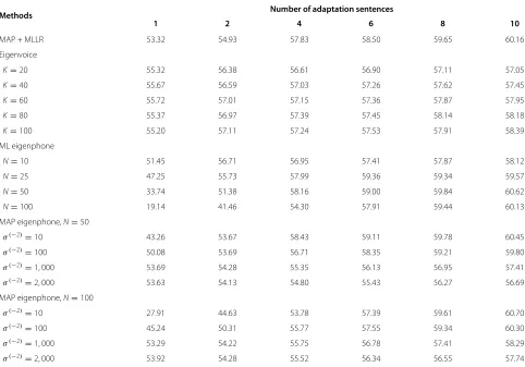
The experiment results of the above methods are sum-marized in Table 1. Significance tests show that when the amount of adaptation data is sufficient (≥ 4 sen-tences) and the number (N) of the eigenphones is 50, the ML eigenphone method outperforms the MAP + MLLR method significantly. But, when the adaptation data is limited to 1 or 2 sentences (about 5∼10 s), the perfor-mance degrades quickly due to over-fitting. The situation is worse when a high-dimensional phone variation
sub-space (i.e.,N = 100) is used. Reducing the number of
the eigenphones improves the recognition rate. However,
even withN = 10, the performance is still worse than
that of the SI model when the adaptation data is one sentence. MAP estimation using a Gaussian prior can alleviate over-fitting to some extent. To prevent perfor-mance degradation, a very small Gaussian prior (i.e., a large weighting factor of the squaredl2norm regularizer)
is required, which heavily limits the performance when there is a sufficient amount of adaptation data available. This suggests that thel2regularization can only improve
the performance in the case of limited amount of adapta-tion data (less than two sentences, about 10 s). In order to demonstrate the performance of the various regular-ization methods, the subsequent experiments all employ a large number of eigenphones, 100.
5.1.3 Eigenphone speaker adaptation using lasso
The lasso regularizer (J(V)withλ1 > 0,λ2 = λ3 = 0) leads to a sparse eigenphone matrix. To measure the sparseness of a matrix, we calculate its ‘overall sparsity’, which is defined as the percentage of nonzero elements
Table 1 Average tonal syllable recognition rate (%) after speaker adaptation using conventional methods
Methods Number of adaptation sentences
1 2 4 6 8 10
MAP + MLLR 53.32 54.93 57.83 58.50 59.65 60.16
Eigenvoice
K=20 55.32 56.38 56.61 56.90 57.11 57.05
K=40 55.67 56.59 57.03 57.26 57.62 57.45
K=60 55.72 57.01 57.15 57.36 57.87 57.95
K=80 55.37 56.97 57.39 57.45 58.14 58.18
K=100 55.20 57.11 57.24 57.53 57.91 58.39
ML eigenphone
N=10 51.45 56.71 56.95 57.41 57.87 58.12
N=25 47.25 55.73 57.99 59.36 59.34 59.57
N=50 33.74 51.38 58.16 59.00 59.84 60.62
N=100 19.14 41.46 54.30 57.91 59.44 60.13
MAP eigenphone,N=50
σ(−2)=10 43.26 53.67 58.43 59.11 59.78 60.45
σ(−2)=100 50.08 53.69 56.71 58.35 59.21 59.80
σ(−2)=1, 000 53.69 54.28 55.35 56.13 56.95 57.41
σ(−2)=2, 000 53.63 54.13 54.80 55.43 56.27 56.69
MAP eigenphone,N=100
σ(−2)=10 27.91 44.63 53.78 57.39 59.61 60.70
σ(−2)=100 45.24 50.31 55.77 57.55 59.34 60.30
σ(−2)=1, 000 53.29 54.22 55.75 56.78 57.41 58.29
σ(−2)=2, 000 53.92 54.28 55.52 56.34 56.55 57.74
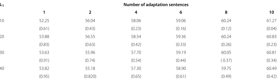
in that matrix. The weighting factor (λ1) of thel1norm
is varied between 10 and 40. The experimental results are summarized in Table 2. For each experiment setting, the average overall sparsity of the eigenphone matrix among all testing speakers is shown in parentheses.
Significance tests show that compared with the ML
eigenphone method, thel1 norm regularization method
can improve the performance significantly. It shows per-formance gain over the MAP eigenphone method under almost every testing condition. The larger the weight-ing factorλ1, the more sparse the resulting eigenphone matrix becomes. When the amount of adaptation data is limited to one, two, four, or six sentences, the best results are obtained withλ1 = 20. The relative improve-ments over the ML eigenphone method are 181.5%, 36.4%, 7.8%, and 2.5%, respectively. When the amount of adap-tation data is increased to eight or ten sentences, a small weighting factor of 10 performs best. The resulting recog-nition rates are still better than that of the ML eigenphone method, with relative improvements of 1.3% and 1.1%, respectively.
5.1.4 Eigenphone speaker adaptation using elastic net For the elastic net method,λ1was fixed to 10. All exper-iments were repeated withλ2changing from 10 to 2,000. The results are summarized in Table 3. Again, the aver-age overall sparsity of the eigenphone matrix is shown in parentheses.
Unfortunately, the results in Table 3 show little improve-ment over the lasso method. The overall sparsity remains the same in all testing conditions. When the adaptation data is one sentence, even with a large weighting fac-tor of l2 = 2, 000, the relative improvement over the
lasso method is only 0.2%. We also set λ1 to different values of 20, 30, and 40, and experimented withλ2 vary-ing from 10 to 2,000. Again, almost no improvement was observed over the results in Table 2. The squaredl2
regu-larization term seems to not work in combination withl1
regularization.
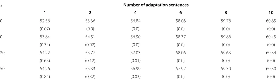
5.1.5 Eigenphone speaker adaptation using group lasso As pointed out in Section 3, the group lasso regularizer leads to a column-wise group sparse eigenphone matrix that is a matrix with many zero columns. To measure the column-wise group sparseness of the eigenphone matrix, we calculate its ‘column sparsity’, which is defined as the per-centage of nonzero columns in that matrix. In the group
lasso experiments, the weighting factor (λ3) of the
column-wisel2norm is varied between 10 and 150. The
results are summarized in Table 4. For each experiment setting, the average column sparsity of the eigenphone matrix among all testing speakers is shown in parentheses. From Table 4, it can be observed that the group lasso method improves the recognition results compared with the ML eigenphone method, especially with limited adap-tation data. Under all testing conditions, its best results are better than that of the MAP eigenphone method, i.e., the squaredl2regularization method. When the
adapta-tion data is limited to one sentence andλ3is larger than 120, the recognition rate is higher than the best results of the lasso method. However, when more adaptation data is provided, the group lasso method no longer achieves bet-ter results than the lasso method. The larger the weighting factorλ3, the larger the column sparsity of the eigenphone matrix. With two adaptation sentences or less,λ3should be larger than 120 to obtain a good row sparsity. With lots of adaptation data (more than four sentences), even with a large value of λ3 of 150, the column sparsity remains very small, that is, almost no column is set to zero. For these nonzero columns, the group lasso is equivalent to the ‘adaptive’l2regularization, and the recognition results
are better than those obtained with the ML eigenphone method.
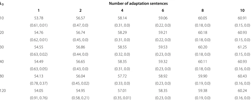
5.1.6 Eigenphone-based speaker adaptation using sparse group lasso
In the sparse group lasso experiments, we fixedλ1to 10 and variedλ3from 10 to 150, in hope that the advantages of the lasso and group lasso methods can be combined.
Table 2 Average tonal syllable recognition rate (%) after eigenphone-based speaker adaptation using lasso
λ1 Number of adaptation sentences
1 2 4 6 8 10
10 52.25 56.04 58.06 59.06 60.24 61.27
(0.61) (0.43) (0.23) (0.16) (0.12) (0.04)
20 53.88 56.55 58.54 59.36 60.24 60.83
(0.83) (0.63) (0.42) (0.33) (0.26) (0.23)
30 53.63 55.96 57.70 59.19 60.05 60.81
(0.91) (0.74) (0.54) (0.44) ( 0.37) (0.34)
40 53.82 55.18 57.30 58.90 59.75 60.49
(0.95) (0.820) (0.65) (0.61) (0.49) (0.42)
Table 3 Average tonal syllable recognition rate (%) after eigenphone-based speaker adaptation using elastic net
λ2 Number of adaptation sentences
1 2 4 6 8 10
10 52.27 55.98 58.10 59.19 60.22 61.08
(0.67) (0.48) (0.33) (0.24) (0.20) (0.16)
40 52.27 55.98 58.14 59.17 60.18 61.08
(0.67) (0.48) (0.33) (0.24) (0.20) (0.16)
80 52.22 55.96 58.12 59.17 60.20 61.04
(0.67) (0.48) (0.33) (0.24) (0.20) (0.16)
120 52.22 55.98 58.16 59.17 60.16 61.08
(0.67) (0.48) (0.33) (0.24) (0.20) (0.16)
1,000 52.31 55.98 58.02 59.13 60.13 60.97
(0.67) (0.48) (0.33) (0.24) (0.20) (0.16)
2,000 52.35 55.98 58.02 59.13 60.16 60.97
(0.67) (0.48) (0.33) (0.24) (0.20) (0.16)
The number of eigenphones (N) was fixed to 100.λ1=10,λ3=0, andλ2was varied between 10 and 2,000. The average overall sparsity is shown in parentheses.
The results are summarized in Table 5. The average overall sparsity and column sparsity of the eigenphone matrix are shown in parentheses.
From Table 5, it can be seen that when the weighting fac-torλ3is set to 20 ∼ 30, the recognition results obtained by applyingl1regularization and the column-wisel2
reg-ularization simultaneously are better than that of using any one of the regularizers. When the amount of adapta-tion data is limited to one and two sentences, the relative improvements over the lasso method are 1.63% and 0.54%, respectively. These results are comparable to that of the best results of the eigenvoice method. When more adap-tation data is available, the relative improvement over the lasso method becomes smaller. However, compared with the group lasso method, the relative improvement is more significant when sufficient adaptation data is pro-vided. The advantages of both thel1regularization and the
column-wisel2regularization combine well. Significance
tests show that withλ1 = 10 andλ3 = 30, the sparse
group lasso is significantly better than all other regulariza-tion methods under all testing condiregulariza-tions.
An interesting phenomenon is observed in that for all experimental settings, the overall sparsity is larger than that of the lasso method, while the column sparsity remains small whenλ3≤40, that is, most of the columns remain nonzero. This observation implies that compar-ing with the lasso method, the performance improvement using the sparse group lasso should be attributed to the wise adaptive shrinkage property of the column-wise unsquaredl2norm regularizer.
5.2 Experiments on the WSJ task
This section gives the unsupervised speaker adaptation results on the WSJ 20K open vocabulary speech recogni-tion task. A two-pass decoding strategy was adopted. For a batch of recognition data from one speaker, hypothesized
Table 4 Average tonal syllable recognition rate (%) after eigenphone-based speaker adaptation using group lasso
λ2 Number of adaptation sentences
1 2 4 6 8 10
60 52.56 53.36 56.84 58.06 59.78 60.85
(0.07) (0.0) (0.0) (0.0) (0.0) (0.0)
90 53.84 54.51 56.90 58.37 59.86 60.45
(0.34) (0.02) (0.0) (0.0) (0.0) (0.0)
120 54.22 55.77 57.03 58.06 59.63 60.34
(0.65) (0.12) (0.01) (0.0) (0.0) (0.0)
150 54.26 55.33 56.99 57.97 59.30 60.30
(0.84) (0.32) (0.03) (0.0) (0.0) (0.0)
Table 5 Average tonal syllable recognition rate (%) after eigenphone-based speaker adaptation using sparse group lasso
λ3 Number of adaptation sentences
1 2 4 6 8 10
10 53.78 56.57 58.14 59.06 60.05 60.91
(0.61, 0.01) (0.47, 0.0) (0.31, 0.0) (0.22, 0.0) (0.18, 0.0) (0.15, 0.0)
20 54.76 56.74 58.29 59.21 60.18 60.93
(0.62, 0.01) (0.45, 0.0) (0.31, 0.0) (0.22, 0.0) (0.18, 0.0) (0.15, 0.0)
30 54.55 56.86 58.55 59.53 60.20 61.25
(0.63, 0.02) (0.44, 0.0) (0.32, 0.0) (0.23, 0.0) (0.18, 0.0) (0.15, 0.0)
40 54.49 56.65 58.35 59.32 60.11 60.93
(0.63, 0.05) (0.43, 0.0) (0.31, 0.0) (0.23, 0.0) (0.18, 0.0) (0.16, 0.0)
80 54.13 56.04 57.72 58.92 59.90 60.43
(0.78, 0.37) (0.45, 0.02) (0.33, 0.0) (0.23, 0.0) (0.19, 0.0) (0.16, 0.0)
120 54.05 54.95 57.01 58.35 59.38 60.24
(0.91, 0.76) (0.58, 0.21) (0.35, 0.01) (0.23, 0.0) (0.19, 0.0) (0.16, 0.0)
The number of eigenphones (N) was fixed to 100.λ1=10.0,λ2=0, andλ3was varied between 10 and 150. the average overall sparsity and column sparsity of the eigenphone matrix are shown in parentheses as pairs.
transcriptions were obtained using the SI model in the first pass. Then, speaker adaptation was performed using the hypothesized transcriptions based on the SI model (without SAT) or the canonical model (with SAT). The final results were obtained in a second decoding pass using the adapted model.
The SI model was trained using the following con-figurations. The standard SI-284 WSJ training set was used for training, which consists of 7,138 WSJ0 ances from 83 WSJ0 speakers and 30,275 WSJ1 utter-ances from 200 WSJ1 speakers. The whole training set contains about 70 h of read speech in 37,413 train-ing utterances from 283 speakers. The acoustic features are the same as that of the Mandarin Chinese task. There were 22,699 crossword triphones based on 39 base phonemes, and these were tree-clustered to 3,339 tied states. At most 16 Gaussian components were estimated for each tied state, resulting in a total of 53,424 Gaussian components.
The WSJ1 Hub 1 development test data (denoted by ‘si_dt_20’ in the WSJ1 corpus) were used for evaluation. For each of the 10 speakers, 40 sentences were selected randomly for testing, resulting in 52 min of read speech in 400 utterances. HDecoder was used as the decoder and the standard WSJ 20K-vocabulary trigram language model was used for compiling the decoding graph. We use word error rate (WER) to evaluate the recognition results. The WER of the SI model is 14.71%.
Unsupervised speaker adaptation was performed with varying amounts of adaptation data. The testing data of each speaker was grouped into batches, with the batch size varying from 2 to 20 sentences. Different batches of data were used for adaptation and evaluation independently.
The following five adaptation methods were tested for comparison:
1. EV: The standard eigenvoice method. 2. MLLR: The standard MLLR method.
3. SAT + MLLR: The standard MLLR method with speaker-adaptive training.
4. EP: The eigenphone method with or without regularization.
5. SAT + EP: The eigenphone method with speaker-adaptive training.
For the eigenvoice method, the number (K) of the eigen-voices was varied between 20 and 150. The best results
were obtained with K = 100 and K = 120 for two
and four adaptation sentences, respectively. When the amount of adaptation data is more than six sentences,
K = 150 yields the best performance. For the MLLR
method, the best results were obtained with a regression class tree using 32 base classes and three-block-diagonal transformation matrices. For the eigenphone method, the dimension (N) of the phone variation subspace was set to 100. Different regularization methods were tested with a wide range of weighting factorsa. Again, the best results
were obtained with the SGL method withλ1 = 10 and
λ3 = 30. The results are summarized in Table 6, where
‘ML-EP’ denotes the eigenphone method with maximum likelihood estimation and ‘SGL-EP’ denotes the SGL reg-ularized eigenphone method. For the sake of brevity, only the best results of each method are shown in the table.
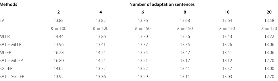
Table 6 Word error rate (%) after unsupervised speaker adaptation on the WSJ task
Methods Number of adaptation sentences
2 4 6 8 10 20
EV 13.88 13.82 13.76 13.68 13.64 13.58
K=100 K=120 K=150 K=150 K=150 K=150
MLLR 14.44 13.86 13.70 13.56 13.43 13.22
SAT + MLLR 13.96 13.41 13.37 13.35 13.26 13.06
ML-EP 16.28 14.24 13.75 13.47 13.41 13.06
SAT + ML-EP 16.80 14.24 13.51 13.17 13.12 12.70
SGL-EP 14.05 13.72 13.52 13.41 13.37 13.00
SAT + SGL-EP 13.92 13.36 13.29 13.11 13.03 12.70
The WER of the SI model is 14.71%. For the sake of brevity, only the best results of each adaptation method are shown in the table. For MLLR, the best results were obtained at a prior weighting factor of 10 (for MAP) and 32 regression classes with a three-block-diagonal transformation matrix (for MLLR). For the eigenphone method, the number of eigenphones (N) was fixed to 100. The weighting factors of the SGL regularization method were set toλ1=10andλ3=30.
methods when more adaptation data become available. The ‘ML-EP’ method outperforms the MLLR method when more than six adaptation sentences are used. Severe over-fitting occurs when the amount of adaptation data is less than four sentences. With sparse group lasso reg-ularization, the robustness of the eigenphone method is improved significantlyb. Compared with the ‘ML-EP’ method, the relative improvements are 13.7%, 3.7%, and 1.7% with two, four, and six adaptation sentences, respec-tively. With more adaptation data, the relative improve-ments are negligible.
Combined with SAT, significant performance improve-ment is observed for all testing methods, except for the ‘SAT + ML-EP’ method with insufficient adaptation data (less than four sentences). Again, the performance degen-eration is due to severe over-fitting. The ‘SAT + SGL-EP’ method performs best under all testing conditions. The relative improvements over the ‘SAT + MLLR’ method and the ‘SAT+ML-EP’ method are 0.3%, 0.4%, 0.6%, 1.8%, 1.7%, and 2.8% and 17.1%, 6.2%, 1.6%, 0.5%, 0.7%, and 0.0% with 2, 4, 6, 8, 10, and 20 adaptation sentences, respectively.
6 Conclusion
In this paper, we investigate various regularization meth-ods to improve the robustness of the estimation of the eigenphone matrix in eigenphone-based speaker adapta-tion. Thel1norm regularization (lasso) introduces
sparse-ness, which reduces the number of free parameters and improves generalization. The squaredl2norm penalizes
large values of the matrix, thus alleviating over-fitting. The
column-wise unsquared l2 norm regularization (group
lasso) forces many columns of the eigenphone matrix to be zero, thus preventing the dimension of the phone variation subspace from being higher than necessary. For nonzero columns, the group lasso is equivalent to
the adaptively weighted column-wise squared l2 norm
regularizer. A unified framework for solving the various regularized matrix estimation problems is presented, and the performances of these regularization methods, includ-ing two combinations of them, i.e., elastic net and sparse group lasso, are compared for a supervised speaker adap-tation task as well as an unsupervised speaker adapadap-tation task using varying adaptation data. Compared with the maximum likelihood estimation method, significant per-formance improvements are observed using any of the regularization methods. Among them, the sparse group lasso method yields best results, which combines the advantages of the lasso and the group lasso methods in a consistent way. The group lasso plays an important role in case of limited amounts of adaptation data, with the performance improvement attributed to its column-wise adaptive shrinkage property. With large amounts of adaptation data, lasso seems to be more important than group lasso. Combined with speaker-adaptive training, performance is further improved.
When the dimension (N) of the phone variation
sub-space is larger than the feature dimension D and the
adaptation data is sufficient, the columns of the
eigen-phone matrix V form an over-complete dictionary. The
corresponding coordinate vector for each Gaussian com-ponent should be sparse. However, the matrixLobtained by PCA will not necessarily show any sparsity. Future work will focus on estimation of a sparse coordinate matrix at training time to obtain more performance gain.
Endnotes
aλ1,λ2andλ3were varied between 0 and 1,000 at a
step size of 10, respectively.
bAgain, all significance tests show that the differences
Abbreviations
DNN, deep neural network; EP, eigenphone; EV, eigenvoice; FISTA, fast iterative shrinkage-thresholding algorithm; HMM, hidden Markov model; HTK, hidden Markov toolkit; IST, iterative shrinkage-thresholding MAP, maximuma posteriori; ML, maximum likelihood MLLR, maximum likelihood linear regression; SA, speaker adapted; SAT, speaker-adaptive training; SD, speaker dependent; SGL, sparse group lasso; SGMM, subspace Gaussian mixture model; SI, speaker independent; SLEP, sparse learning with efficient projections.
Competing interests
The authors declare that they have no competing interests.
Acknowledgements
This work was supported in part by the National Natural Science Foundation of China (No. 61175017 and No. 61005019) and the National High-Tech Research and Development Plan of China (No. 2012AA011603). The authors would like to thank the anonymous reviewers and Prof. Michael T. Johnson for their valuable suggestions that improved the presentation of the paper.
Author details
1Zhengzhou Information Science and Technology Institute, Zhengzhou
450000, China.2Tsinghua National Laboratory for Information Science and Technology, Department of Electronic Engineering, Tsinghua University, Beijing 100084, China.
Received: 16 June 2013 Accepted: 21 March 2014 Published: 5 April 2014
References
1. R Kuhn, JC Junqua, P Nguyen, N Niedzielski, Rapid speaker adaptation in eigenvoice space. IEEE Trans. Speech Audio Process.8(6), 695–707 (2000) 2. MJF Gales, Maximum likelihood linear transformations for HMM-based
speech recognition.Comput. Speech Lang.12(2), 75–98 (1998) 3. WL Zhang, WQ Zhang, BC Li,Speaker adaptation based on
speaker-dependent eigenphone estimation. (Paper presented at the IEEE Workshop on automatic speech recognition and understanding, Waikoloa, HI, 11–15 Dec 2011), pp. 48–52
4. P Kenny, G Boulianne, P Ouellet, P Dumouchel, Speaker adaptation using an eigenphone basis. IEEE Trans. Speech Acoust. Process.12(6), 579–589 (2004)
5. QF Tan, PG Georgiou, SS Narayanan, Enhanced sparse imputation techniques for a robust speech recognition front-end. IEEE Trans. Acoust. Speech Signal Process.19(8), 2418–2429 (2011)
6. L Lu, A Ghoshal, S Renals, Regularized subspace Gaussian mixture models for speech recognition. IEEE Signal Process. Lett.18(7), 419–422 (2011) 7. F D Yu, G Seide, L Li,Deng, Exploiting sparseness in deep neural networks for
large vocabulary speech recognition. (Paper presented at ICASSP, Kyoto, Japan, 25–30 Mar 2012), pp. 4409–4412
8. QF Tan, SS Narayanan, Novel variations of group sparse regularization techniques with applications to noise robust automatic speech recognition. IEEE Trans. Acoust. Speech Signal Process.20(4), 1337–1346 (2012)
9. DQu WL Zhang, WQ Zhang, BC Li. Rapid speaker adaptation using compressive sensing.Speech Commun.55(10), 950–963 (2013) 10. WL Zhang, WQ Zhang, DQu BC Li, MT Johnson, Bayesian speaker
adaptation based on a new hierarchical probabilistic model. IEEE Trans. Audio Speech Lang. Process.20(7), 2002–2015 (2012)
11. J T Anastasakos, R McDonough, J Schwartz, A Makhoul, compact model for speaker-adaptive training. Paper presented at the ICSLP, Philadelphia, PA. USA, 3–6, 1137–1140 (Oct 1996)
12. CH Lee, CH Lin, BH Juang, A study on speaker adaptation of the parameters of continuous density hidden Markov models. IEEE Trans. Acoust. Speech Signal Process.39(4), 806–814 (1991)
13. CJ Leggetter, PC Woodland,Flexible speaker adaptation using maximum likelihood linear regression. (Paper presented at the ARPA spoken language technology workshop, 22–25 Jan 1995), pp. 110–115
14. R Tibshirani, Regression shrinkage and selection via the LASSO. J. R. Stat. Soc. (Ser. B).58, 267–288 (1996)
15. R T Hastie, J Tibshirani,Friedman, The Elements of Statistical Learning: Data Mining, Inference and Prediction. (Springer, Berlin, 2005)
16. M Yuan, Y Lin, Model selection and estimation in regression with grouped variables. J. R. Stat. Soc. (Ser. B).68, 49–67 (2007)
17. H Zou, T Hastie, Regularization and variable selection via the elastic net. J. R. Stat. Soc. B (Stat. Methodol.)67(2), 301–320 (2005)
18. N Simon, J Friedman, T Hastie, R Tibshirani, A sparse-group lasso. J. Comput. Graph. Stat.22(2), 231–245 (2013)
19. JF Gemmeke, T Virtanen, A Hurmalainen, Exemplar-based sparse representations for noise robust automatic speech recognition. IEEE Trans. Acoust. Speech Signal Process.19(7), 2067–2080 (2011) 20. M Figueiredo, R Nowak, S Wright, Gradient projection for sparse
reconstruction: application to compressed sensing and other inverse problems. IEEE J. Sel. Top. Signal Process.1(4), 586–597 (2007) 21. J Liu, S Ji, J Ye,SLEP: Sparse Learning with Eefficient Projections. (Arizona
State University, Tempe, 2009)
22. A Beck, M Teboulle, A fast iterative shrinkage-thresholding algorithm for linear inverse problems.SIAM. J. Imaging Sci.2, 183–202 (2009) 23. E Richard, PA Savalle,Estimation of simultaneously sparse and low rank
matrices. (Paper presented at the ICML, 26 June – 1 July 2012), pp. 1351–1358
24. DP Bertsekas, Incremental proximal methods for large scale convex optimization. Math. Program.129(2), 163–195 (2011)
25. D Blatt, AO Hero, H Gauchman, A convergent incremental gradient method with a constant step size.SIAM. J. Optim.18, 29–51 (2008) 26. N Parikh, S Boyd. Proximal algorithms.Foundations Trends Optimization.
1(3), 1–108 (2013)
27. Y Nesterov, A method of solving a convex programming problem with convergence rateO1
k2
. Sov. Math. Doklady.27, 372–376 (1983)
28. I Daubechies, MD Friese, CD Mol, An iterative thresholding algorithm for linear inverse problems with a sparsity constraint.Comm. Pure Appl. Math. 57, 1413–1457 (2004)
29. E Chang, Y Shi, J Zhou, C Huang, Speech lab in a box : a Mandarin speech toolbox to jumpstart speech related research. Aalborg, Denmark, 2799–2802 (3–7 Sept 2001)
30. The National Institute of Standards and Technology the NIST Scoring Toolkit (SCTK-2.4.0). ftp://jaguar.ncsl.nist.gov/pub/sctk-2.4.0-20091110-0958.tar.bz2. Accessed 25 Sept 2013
31. G S Young, M Evermann, T Gales, D Hain, X Kershaw, G Liu, J Moore, D Odell, V Ollason, P Valtchev,Woodland, The HTK Book (for HTK Version 3.4). (Cambridge University Engineering Department, Cambridge, 2009) 32. VV Digalakis, LG Neumeyer, Speaker adaptation using combined
transformation and Bayesian methods. IEEE Trans. Speech Audio Process. 4(4), 294–300 (1996)
doi:10.1186/1687-4722-2014-11
Cite this article as:Zhanget al.:Speaker adaptation based on regularized speaker-dependent eigenphone matrix estimation. EURASIP Journal on Audio, Speech, and Music Processing20142014:11.
Submit your manuscript to a
journal and benefi t from:
7Convenient online submission 7Rigorous peer review
7Immediate publication on acceptance 7Open access: articles freely available online 7High visibility within the fi eld
7Retaining the copyright to your article