R E S E A R C H
Open Access
Stereo-based histogram equalization for
robust speech recognition
Randa Al-Wakeel
1*, Mahmoud Shoman
2, Magdy Aboul-Ela
1and Sherif Abdou
2Abstract
Optimal automatic speech recognition (ASR) takes place when the recognition system is tested under
circumstances identical to those in which it was trained. However, in the actual real world, there exist many sources of mismatches between the environment of training and the environment of testing. These sources can be due to the sources of noise that exist in real environments. Speech enhancement techniques have been developed to provide ASR systems with the robustness against the sources of noise. In this work, a method based on histogram equalization (HEQ) was proposed to compensate for the nonlinear distortions in speech representation. This approach utilizes stereo simultaneous recordings for clean speech and its corresponding noisy speech to compute stereo Gaussian mixture model (GMM). The stereo GMM is used to compute the cumulative density function (CDF) for both clean speech and noisy speech using a sigmoid function instead of using the order statistics that is used in other HEQ-based methods. In the implementation, we show two choices to apply HEQ, hard decision HEQ and soft decision HEQ. The latter is based on minimum mean square error (MMSE) clean speech estimation. The experimental work shows that the soft HEQ and hard HEQ achieve better recognition results than the other HEQ approaches such as tabular HEQ, quantile HEQ and polynomial fit HEQ. It also shows that soft HEQ achieves notably better recognition results than hard HEQ. The results of the experimental work also show that using HEQ improves the efficiency of other speech enhancement techniques such as stereo piece-wise linear compensation for environment (SPLICE) and vector Taylor series (VTS). The results also show that using HEQ in multi style training (MST) significantly improves the ASR system performance.
Keywords:Robust speech recognition; Speech feature normalization; Histogram equalization; Speech enhancement
1 Introduction
Optimal automatic speech recognition (ASR) takes place when the recognition system is used under circum-stances identical to those in which it was trained. How-ever, in the actual real world, there exist many sources of mismatches between the environment of training and the environment of testing. These mismatches can be due to the sources of noise which include additive noise, linear filtering, and nonlinearities in transduction or transmission, as well as impulsive interfering. For this reason, robust speech recognition in noisy environments is one of the focus areas of speech research [1, 2]. The objective of robustness techniques is to provide ASR systems with robustness against the noise sources.
Most ASR systems are trained using training data recorded in typical clean conditions. However, in real environments, the noise introduces a distortion in the feature space and due to its random nature, it causes a loss of information [1]. It usually produces a nonlinear transformation of the feature space depending on the speech representation and the type of noise. For ex-ample, in the case of cepstral-based representations, additive noise causes a nonlinear transformation that has no significant effect on high-energy frames but a strong effect on those with energy levels in the same range or below that of the noise. Many speech enhance-ment techniques assume that the distortion is a function in clean speech and noise sources. Such that the noisy speech can be expressed as:
yt ¼xtþf xð t;nt;htÞ * Correspondence:[email protected]
1
Sadat Academy for management Science and Information Systems, Cairo, Egypt
Full list of author information is available at the end of the article
where tis the time frame index, xt,yt, and ntare the
clean, noisy, and additive noise Mel frequency cepstral coefficients (MFCC) vectors, respectively, and ht is the
corresponding convolutional noise vector. The random nature of the additive and convolutional noises results in one to many mappings between clean and noisy feature spaces and a given clean feature vector can generate different noisy vectors, and vice versa [3].
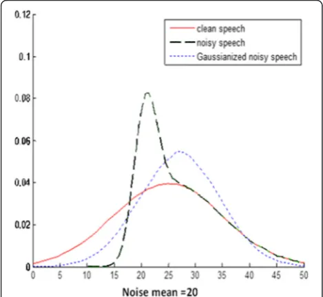
Figure 1 shows the effect of noise on the probability density function of clean speech when the noise is as-sumed stationary Gaussian noise [2]. The clean speech has a mean value of 25 and a standard deviation of 10. The noise has a standard deviation of 2. In general, the convolutional noise mainly shifts the mean of the coeffi-cients, whereas additive noise modifies the probability density function (PDF), reducing the variance of the co-efficients [3].
Speech enhancement techniques aim to achieve the robustness of the ASR systems in noisy environments. Speech enhancement methods can be classified into two main categories [2]. The first category is feature-domain-based methods which in turn have been classified into three approaches, noise resistant features, feature normalization, and feature compensation. The second main category is the model-domain methods. In noise-resistant feature approach, robust signal processing is employed to reduce the sensitivity of the speech fea-tures to the environment conditions that do not match those used to train the acoustic model. Examples of noise-resistant features include PLP [4, 5] and zero-crossing peak amplitude (ZCPA) [6], average localized synchrony detection (ALSD) [7], and perceptual
minimum variance distortionless response (PMVDR) [8]. Although these features can usually achieve better performance than MFCC [9] which is popular in most of ASR systems, they have a much more complicated generation process which sometimes prevents them from being widely used together with some noise ro-bustness technologies.
Feature moment normalization techniques normalize the statistical moments of speech features. Cepstral mean normalization (CMN) [10] is one of the most popular feature moment normalization techniques. It is involved in most speech recognition systems. It effi-ciently reduces the effects of unknown linear filtering in the absence of additive noise by subtracting the mean of the cepstral coefficients in order to remove the global shift of the mean in the cepstral vectors [1]. Another technique of moment normalization is cepstral mean and variance normalization (CMVN) [11]. CMVN nor-malizes the second-order statistical moments. Also, histogram equalization (HEQ) [1] is classified as one of this category of methods. It normalizes the higher statis-tical moments through the feature histogram.
The third subcategory of feature domain speech en-hancement is feature compensation which aims to re-move the effect of noise from the observed speech features. So, a clean version of the speech is recognized using the clean models. They include, but are not lim-ited to, spectral subtraction (SS) [12], vector Taylor series (VTS) [13], stereo piece-wise linear compensation for environment (SPLICE) [14], and stereo-based sto-chastic vector mapping (SSM) [15, 16].
The second main category is the model-space methods [17, 18]. This class of methods attempts to modify the acoustic model parameters to incorporate the effects of noise in order to allow them to represent noisy speech properly. So the noisy speech is recognized using noisy models [19, 20]. Model space methods only adapt the model parameters to fit the distorted speech signal. The model adaptation can operate in either supervised or unsupervised mode. In supervised mode, the correct transcription of the adapting speech utterance is avail-able. It is used to guide model adaptation to obtain adapted model which is used to decode the incoming utterances. In unsupervised model, the correct tran-scription is not available. Two-pass decoding is usually used. In the first pass, the initial model is used to de-code the utterance to generate a hypothesis. And then the updated model is obtained and used to generate the final decoding result [2]. While typically achieving higher accuracy than feature-domain methods, they usually incur significantly higher computational cost. In addition, this class of methods needs a large amount of adaptation data. This may be difficult to be available in many situations.
Speech enhancement techniques may use a single chan-nel recording such as VTS and spectral subtraction or multi-channel recordings such as SSM and SPLICE.
In this work, we are interested in the HEQ method used to compensate for the nonlinear distortions in speech representation. HEQ has a set of advantages. It can be applied in the feature domain, independently from the recognizer back end, without the need for a prior information about typical noise or the signal-to-noise ratio (SNR) to be expected and does not require voice activity detection (VAD) to estimate noise. Also, it is computationally inexpensive. In addition to these ad-vantages, since it can be considered as a feature normalization technique, it can be applied before or after other speech enhancement techniques such as SPLICE and VTS approaches.
In this work, we utilize stereo simultaneous recordings for the clean and the corresponding noisy speech in order to train stereo Gaussian mixture model (GMM). The stereo GMM model is used to compute cumulative density function (CDF) tables for both clean and noisy speech. The CDF values are computed using sigmoid function. We aim to evince the effectiveness of the pro-posed HEQ method when it is applied either alone or in combination with VTS and SPLICE approaches. In addition, we aim to demonstrate its effectiveness when it is used in a process of multi-style training of the acoustic recognition models and using the resulted model to recognize speech processed by HEQ.
The paper is organized as follows. Section 2 reviews the main theory of HEQ. Three HEQ-based approaches are described. Section 3 introduces a speech enhance-ment approach based on HEQ. This method depends on the availability of stereo recordings for the training clean speech and its corresponding noisy speech. Two ap-proaches to implement HEQ are presented, the hard decision HEQ and the soft decision HEQ. The experi-mental work and results are shown in Section 4, and fi-nally, in Section 5, the conclusions and future work are presented.
2 Theory of histogram equalization
The acoustic mismatch between clean reference features and noisy test features caused by the environmental noise produces a statistical difference between their cor-responding probability density functions (PDFs) [21]. HEQ attempts to transform the PDF of the original test (noisy) feature into its reference (or training) PDF [22–24] to improve the recognition accuracy. In the implemen-tation of HEQ, reference and test PDFs are replaced by their corresponding reference histograms and the test histogram. The main objective is to find the transform-ation which achieves the equaliztransform-ation of the CDF of the noise observed coefficient to the CDF of the clean
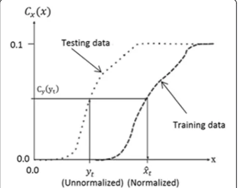
coefficient. HEQ is applied to each feature on a component-by-component basis. The principle of HEQ can be clarified using Fig. 2 [25].
Let the random variableywith pdfp(y) and CDFCy(y)
can be transformed to a random variable ^x¼ Txð Þy
with a probability density functionϕxð Þ^x and CDFCxð Þx^ which is identical to that of the reference CDF, such as:
Cyð Þ ¼y Cxð Þx^ ð1Þ
So the estimated clean speech coefficient can be ob-tained by applying the inverse of the reference cumula-tive density function on the noisy CDF:
^
x¼ C−x1 Cyð Þy
ð2Þ
This process is assumed to transform the test data distribution into the training data distribution.
Clearly, the effectiveness of HEQ is directly related to the reliable estimation of both reference and test CDFs [26]. CDF can be estimated efficiently by using a large amount of sample data. This amount of data can be ob-tained at the training phase. So, the reference CDF can be obtained quite reliably. On the other hand, at the test phase, when short utterances are to be recognized, the amount of sample data may be insufficient for the reli-able estimation of the test CDF. In this case, many re-searches [27, 24, 25] used the order statistics to compute the test CDF.
2.1 Computing CDF using order statistics
LetWbe the test utterance to be recognized.Wconsists
of N frames. Since HEQ works in a
component-by-component basis, thekth component in all theNframes
is considered. This sequence of values of thekth compo-nent over all theNframes can be denoted as:
Yk¼ ykð Þ1 ;ykð Þ2 ;………;ykð ÞN
ð3Þ
The first step is to sort this sequence of values in as-cending order such that [24]:
ykð Þ½ 1 ≤…≤ykð½ rkÞ≤…≤ykð½ NÞ ð4Þ
where [rk] and rkdenote the original frame index of
fea-ture component y([rk]), and its rank (respectively) when
the elements of the sequenceYkare sorted in ascending
order. The order statistics-based estimate of the test CDF is as follows:
CYk yk½ rk
¼ rk−0:5
N ð5Þ
This is the principle of HEQ speech enhancement ap-proach. Speech enhancement methods based on HEQ have implemented HEQ in a variety of ways.
2.2 Variations of HEQ
We will briefly describe three effective HEQ-based ap-proaches in this section.
2.2.1 Table-based histogram equalization (THEQ)
THEQ [28] is a non-parametric method to make the dis-tributions of the test speech match those of the training speech. The cumulative histogram is used to estimate the corresponding CDF value of each feature vector
component y. It has two phases. The first phase is the
training phase, in which the cumulative histogram of each feature vector component of the training data is computed resulting in a table of the CDF values for a
number ofKbins between the maximum and minimum
values of each feature component.
The second phase is the table look-up process in which the restored value of each feature vector
com-ponent x of the test utterance is obtained by using
its estimated CDF value as the key to finding the corresponding transformed (restored) value in the CDF table [29].
2.2.2 Quantile-based histogram equalization (QHEQ)
Instead of the full match of the cumulative histogram that is implemented by THEQ, QHEQ [30, 3] uses a quantile-corrective manner to calibrate the CDF of each feature vector component of the test speech to that of the training speech [29]. In QHEQ, a transformation function is estimated by minimizing the mismatch be-tween the quantiles of the test utterance and those of the training data. The transformation function is then
applied to each feature component x to make the CDF
of the equalized component match that observed in
training. The estimation of the transformation function can be implemented using a single test utterance (or ex-tremely, a very short utterance), without the need of an additional set of adaptation data [3]. On the other hand, in order to find the optimum transformation parameters for each feature vector component, an exhaustive online grid search is needed. This search process is very time-consuming [29].
2.2.3 Polynomial-fit histogram equalization (PHEQ)
PHEQ uses the data fitting scheme to efficiently approxi-mate the inverse functions of the CDFs of the training speech for HEQ [29]. Data fitting is a method for math-ematical optimization. This method takes a series of data points(ui,vi)withi= 1,…,Nand attempts to find a
func-tion G(ui) whose output ṽi closely approximates vi by
minimizing the sum of the squares error between the points (ui, ṽi) and their corresponding points (ui,vi) in
the data.N is the number of points. The functionG(ui)
to be estimated can be either linear or nonlinear in its coefficients.
Such data fitting (or so-called least squares regression) is used in PHEQ to estimate the inverse functions of the CDFs of the training speech. For each speech feature vector component of the training data, given the pair of the CDF value CTrain(yi) of the vector componentyiand
yiitself, the linear polynomial functionG(CTrain(yi)) with
outputỹican be expressed as:
G Cð Trainð Þyi Þ ¼ ~yi¼ XS
s¼0
asðCTrainð Þyi Þs ð6Þ
where the coefficientsascan be estimated by minimizing
the squares error expressed in the following equation:
E2¼ X N
i¼1
yi−~yi ð Þ2
¼XN i¼1
yi− XS
s¼0
asðCTrainð Þyi Þs !2
ð7Þ
Here, N denotes the total number of training speech
feature vectors, and S is the order of the polynomial
function.
3 Histogram equalization using stereo databases
In this work, stereo training database (i.e., data that con-sists of simultaneous recordings of both the clean and noisy speech) is used to build stereo Gaussian mixture model (GMM) which is used to estimate both the refer-ence CDF and the test CDF of each feature vector com-ponent. The proposed HEQ method uses CDF tables which are computed using stereo GMM which models the joint PDF of clean-noise speech. In addition, the method estimates the clean speech feature using a mini-mum mean square error (MMSE) criterion. Two ap-proaches to apply HEQ, hard decision HEQ and soft decision HEQ, are investigated.
Stereo databases were used with HEQ in earlier work in [31]. In [31], the stereo database was used to train two separated GMM models, one to model the test en-vironment and the other to model the clean speech. The two models are used to estimate the clean speech in a MMSE framework.
In this work, the stereo database is used to train a stereo GMM by concatenating each clean speech frame together with the corresponding noisy speech feature vector. Another difference is that cumulative density function tables for both clean and noisy speech are computed using the sigmoid function that utilizes the stereo GMM, so the order statistics is not used to com-pute the test CDF.
The following sections describe the details of imple-menting the proposed approach.
3.1 The joint probability distribution
The joint distribution is built using the stereo database. Letx= (x1,x2,...,xK) be the clean feature vector whereK
is the dimension of the vector. The corresponding sim-ultaneously recorded noisy representation is y= (y1,
y2,...,yK)
Definez≡(x,y) as the concatenation of the two chan-nels. So the dimension ofzis 2*K.
Gaussian mixtures are used to model the joint prob-abilityp (z).So,p (z)can be estimated as:
p zð Þ ¼X M
m¼1
cmN z;μz;m;Σzz;m
ð8Þ
where M is the number of mixture components, cm,
μz,m, andΣzz,mare the mixture weight, mean, and
covari-ance of the mth component, respectively. Also, both the mean and covariance can be partitioned as
μz;m¼ μx;m μy;m
ð9Þ
Σzz;m¼ ΣΣxx;m Σxy;m yx;m Σyy;m
ð10Þ
The GMM model can be trained using the expectation maximization (EM) algorithm [32].
3.2 The use of sigmoid function to approximate CDF values
As mentioned above, the efficiency of HEQ approach is directly related to the reliable estimation of the CDF values. So, our objective now is to find a reliable method to estimate the CDF values given the stereo GMM.
In probability theory and statistics, the logistic dis-tribution [33] is a continuous probability disdis-tribution resembles in its shape the Gaussian distribution and its cumulative distribution function has a similar shape as the CDF of the Gaussian distribution but it has heavier tails (higher kurtosis). The CDF of logistic
distribution at the point x is computed using the
fol-lowing formula:
Clð Þ ¼x
1
1þ exp −ðx−μlÞ σl
h i ð11Þ
where μl and σl are the mean and the standard
devi-ation of the logistic distribution.
In this work, a formula similar to (11) is used to com-pute the CDF values using the mean and standard devi-ation of the stereo GMM.
3.3 HEQ using stereo GMM and sigmoid function
In HEQ, it is assumed that speech features are statistically independent, so it works in a component-by-component basis. The proposed HEQ approach is implemented in two phases. In the first phase, tables for the CDF values are computed using the stereo GMM both for the clean speech and noisy speech. In the second phase, the CDF ta-bles are used to transform the observed noisy coefficient to its clean estimate.
1) Calculating the CDF tables: using each Gaussian mixturem, 1 ≤ m ≤M, and for each component k, 1 ≤k ≤K, the cumulative histogram is estimated by considering a large number of bins V(e.g., 100) uniform intervals calculated between
μm− 4σm andμm + 4σm whereμm is the mean
andσm is the standard deviation of the
component at mixturem.
Qv¼
1
1þγexp v−μm σm
h i ð12Þ
The parameterγis a constant, and its value is chosen experimentally so the approximated HEQ transform-ation is smooth.
This process is implemented for both clean part and noisy part of the stereo GMM mixture. In the
following, the notationQvc is used to denote the CDF
for the clean part and Qvn is used to denote the CDF
of the noisy part. At the end of this phase, the CDF tables for clean and noisy parts of the GMM are ob-tained. The tables contain pairs of the bins and their corresponding CDF values. Each (bin, CDF) pair is denoted by (v, Qv).
4 Applying HEQ to the test speech
For each component yk in the observed speech feature
vectory, the clean speech estimate can be calculated using
Gaussian mixture m as follows. The noise CDF table is
used to detect the interval to which the componentyk
be-longs. So, we want to find the nearest two binsvn
i andvniþ1 to the componentyk, soyk∈ vni; vniþ1
.
The value of the cumulative density function atykC(yk) is
computed as a linear interpolation of their CDF values as:
C yk ¼ Qvni þQvniþ1
2 ð13Þ
where 1≤i≤V.
The computed CDFC(yk) is used to estimate the clean
speech feature^xusing the clean CDF table, such that
^ x¼ v
c jþ vcjþ1
2 ð14Þ
where vcj and vcjþ1 are the values of the bins whose CDF values are the nearest toC(yk).
However, in practice, there is no way to decide which
mixture the observed speech vector y belongs to. Two
choices were investigated:
1. Hard decision-based HEQ: in this approach, the mixturemwhosep(y|m) is maximum, is selected:
^
m¼ arg max
1≤m≤Mp Yð jmÞ ð15Þ
So, the HEQ is implemented using the CDF tables which are related to mixturem^:
2. Soft decision-based HEQ: in this approach, the HEQ algorithm is applied using all the mixtures. The clean speech estimate is computed in a minimum mean square error (MMSE) basis using
^
x¼E x½ jy ð16Þ
The main assumption is that the speech features are statistically independent. So, in the following, we will de-note the speech feature asxfor clean speech feature and y for noisy speech feature to indicate they are scalars. Considering the GMM structure of the joint distribu-tion, Equation (16) can be further decomposed to:
^ x¼
Z
x
p xð Þjy xdx¼X m
Z
x
p x;ð mjyÞxdx
^
x¼X
m
p mð jyÞ
Z
x
p x;ð mjyÞxdx
¼X
m
p mð jyÞ
Z
x
p xð jm;yÞxdx
¼X
m
p mð jyÞE x½ jm;y
ð17Þ
Considering thatE[x|m,y] is equal to the clean speech estimate computed in (14), and setting it as,
~
xm ¼E x½ jm;y ð18Þ
so we reach the following equation,
~
xm ¼E x½ jm;y ð19Þ
where p(m|y) is the posterior probability of the
mix-turemgiven the observed vector y. It can be computed
by:
p mð jyÞ ¼ Xp yMð jmÞp mð Þ m¼1p yð jmÞp mð Þ
ð20Þ
Soft-HEQ approach requires computing (14)M times,
where M is the number of mixtures, while for hard
HEQ, Equation (14) is computed only once (for the mix-ture withp(Y|m) is maximum). So, for each component, soft HEQ requiresM(M+ 1) multiplications andM2 ad-ditions more than hard HEQ. This computational cost can be neglected when the number of mixtures is not large.
5 Experimental work and results
close-taking microphone and a 16-channel array of first-order hypercardiod microphones mounted on the visor. Data from two channels only are used. The first one is the close-talking microphone (CT) channel. The second one is a single channel from the microphone array, re-ferred to as hands-free data (HF) henceforward. The average SNR is about 21 db for the CT channel and 8 db for the HF channel. The experiments were implemented using the part of the database that contains only the digit utterances.
The data are recorded at 24-kHz sampling rate and are down sampled to 8 kHz. They are then windowed with 12.5 ms frame rate and 25 ms frame size. Filter bank analysis is then applied. The filter bank has 26 channels. MFCCs are calculated by applying DCT to log filter bank amplitudes to produce 12 cepstral coeffi-cients. The energy coefficients are also computed and appended to the cepstral vectors. Therefore, each ceps-tral vector contains 13 coefficients. During recognition, delta and delta-delta coefficients are computed on the fly resulting in vectors of 39 coefficients.
We have implemented speech enhancement using Gaussian mixtures models with sizes 16, 64, and 256 mixtures.
The recognition models for digits are trained using about 6500 training clean speech files collected from the CT microphone and tested using about 800 utterances. For each digit from 0 to 9, there is a hidden Markov model (HMM). The digit 0 has an additional model for the utterance“oh.”A 12th model is considered to model silence. Each of these models consists of 6 states. Each state contains 8 mixtures. The clean speech files are also used to build the clean speech Gaussian mixture models that were used in the experiments. Training and recog-nition is done using HTK [34].
In the HEQ experiments, constantγused in the
com-putation of the CDF in (12) takes the value−1.7.
A baseline set of results for this task is given in Table 1.
This table shows the evaluation of the recognition sys-tem in the different test/train conditions. In terms of sentence error rate (SER), Clean refers to the CT chan-nel and noisy refers to the HF chanchan-nel.
The first result shows the SER when clean speech is recognized using systems trained using clean database. The second result shows the result when the recognition system is trained and tested using noisy speech. The
error rate is low in the two cases. This is because the en-vironment of testing is similar to the enen-vironment of training. However, when the system is trained using clean speech and tested using noisy speech the recogni-tion performance degrades severely. This is clear in the third experiment of Table 1 which shows how the system would perform in practical situations when the system is trained using clean speech and tested using observed speech. We can see dramatic degradation in performance due to the noise, 31.72 SER in noisy environment vs. 12.94 SER in clean environment.
Applying compensation techniques to the noisy speech improves the recognition results.
The SPLICE, VTS, and HEQ are applied to the MFCC coefficients before CMN. After applying the compensa-tion, CMN was performed then the delta and delta-delta coefficients were computed.
Table 2 shows the results obtained by applying SPLICE and first-order vector Taylor series (VTS) technique.
We see that the best result obtained with the number of mixtures is 256. In this case, SPLICE represents about 13 % relative improvement to the baseline, and VTS rep-resents about 9 % relative improvement.
The next set of experiments test the performance of the proposed hard and soft HEQ approaches in compari-son with THEQ, QHEQ, and PHEQ approaches. Table 3 shows the results of these experiments.
From results in Table 3, we can see that the proposed approach outperformed the other HEQ approaches which did not provide significant improvement com-pared with the baseline system. Also, we can see the su-periority of soft HEQ over the hard HEQ approach which achieved a relative 25.5 % reduction in SER over the baseline using 64 mixtures while the hard decision HEQ achieved only 9 % relative improvement in the SER using 256 mixtures.
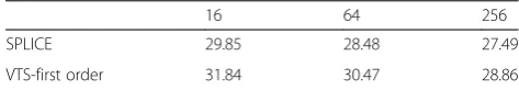
The next set of experiments tested the effect of com-bining soft HEQ with other speech enhancement methods. Table 4 shows the results of applying SPLICE and VTS speech enhancement methods to the soft HEQ processed noisy speech.
From results shown in Table 4, we can see that apply-ing SPLICE and VTS after HEQ achieves better results than the case when the SPLICE and VTS are applied dir-ectly on the noisy speech. Applying HEQ to the noisy speech before SPLICE introduces improvement to the performance of SPLICE by about 16 %. And in case of
Table 1The base line recognition results
Condition SER
Clean/Clean 12.94
Noisy/Noisy 16.79
Clean/Noisy 31.72
Table 2SER after SPLICE and VTS speech enhancement
16 64 256
SPLICE 29.85 28.48 27.49
VTS, the improvement was about 13.6 % of the SER ob-tained by VTS alone.
In the last set of experiments, the soft HEQ was evalu-ated with the multi style trained (MST) recognition models. This is done in two steps:
a) Applying soft HEQ to the noisy training data to yield HEQ enhanced speech.
b) Constructing the training database by merging the clean speech database with the SSM-enhanced speech database. The new database is used to train the recognition models.
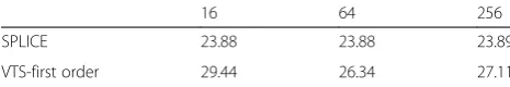
The resulted models are used to recognize HEQ proc-essed noisy speech and noisy speech procproc-essed by THEQ, QHEQ, PHEQ, soft HEQ followed by VTS, and soft HEQ followed by SPLICE. Table 5 shows the results of these experiments.
The first row of Table 5 shows the SER obtained when the noisy unprocessed speech is recognized using multi-style trained recognition models.
The next three rows show the SER when the noisy speech is processed by THEQ, QHEQ, and PHEQ and then recognized by the multi-style trained HMM model. The last three rows show the SER when the soft HEQ is applied alone and with SPLICE and VTS speech en-hancement methods.
THEQ, QHEQ, and PHEQ approaches achieve only 13.55, 13.46, and 15.5 % (respectively) improvements in the SER relative to the baseline. However, in case of 64 mixtures, the improvement in the SER achieved in case of MST when the noisy speech is processed by only soft HEQ was about 50 % relative to the baseline. When the noisy speech is processed by HEQ then by SPLICE the improvement was 48.6 % in case of 64 mixtures and this percentage is decreased when the number of mixtures increased to 256. When the noisy speech is processed by HEQ then by VTS, the improvement was about 39 %.
The results of the experiments also show that the im-provement achieved when the soft HEQ is implemented alone is better than the case when it is combined with SPLICE and VTS which provide a computationally an effective noise reduction approach.
6 Conclusions
In this paper, we proposed a speech enhancement-method based on HEQ. HEQ attempts to eliminate the nonlinear distortions of noise by transforming the PDF of the ori-ginal noisy feature into its reference training PDF to im-prove the recognition performance. In this work, we used stereo speech recordings to build stereo GMM to model the joint probability of clean and noisy speech. The stereo GMM is used to compute the CDF tables using the sig-moid function. Two approaches to implement the HEQ method were investigated. The first is hard decision HEQ and the second is soft decision HEQ. The experimental work shows that soft decision HEQ notably achieves bet-ter speech recognition results than hard decision HEQ. Both soft HEQ and hard HEQ provided better perform-ance than the other HEQ approaches such as THEQ, QHEQ, and PHEQ using clean speech trained and multi-style trained recognition models.
Also, the HEQ approach achieves better performance than SPLICE and VTS methods and applying HEQ to the noisy speech before SPLICE and VTS speech en-hancement methods improves the performance of such enhancement methods but did not achieve better results than the results of applying HEQ alone.
The best recognition results are obtained when using number of mixtures in the GMM equal to 16. When used larger number of mixtures, the percentage of achieved performance improvement decreases. May using larger training data set provide better perform-ance for larger number of mixtures?
Finally, more improvements to the recognition per-formance of ASR are obtained when the HEQ is used to enhance a set of noisy speech and incorporating this new speech data to the training speech corpus in a multi style training framework.
Table 3SER after histogram equalization
16 64 256
THEQ 31.43
QHEQ 31.68
PHEQ 30.39
Hard HEQ 29.85 29.85 28.86
Soft HEQ 26.87 23.63 24.38
Table 4SER SPLICE and VTS compensation applied on soft
histogram equalized speech
16 64 256
SPLICE 23.88 23.88 23.89
VTS-first order 29.44 26.34 27.11
Table 5SER after HEQ evaluated by multi-style trained recognition
models
16 64 256
Noisy unprocessed 27.49
THEQ 27.42
QHEQ 27.45
PHEQ 26.88
Soft HEQ 16.42 15.8 17.41
Soft HEQ then VTS 20.27 19.47 19.4
It is obvious that histogram normalization is computa-tionally attractive as it does not require a process of noise estimation before applying the enhancement ap-proach such as VTS. It also does not need the computa-tion of correccomputa-tion vectors like SPLICE. In addicomputa-tion, since HEQ is implemented in a component-by-component manner, it does not require matrix operations in its im-plementation which is very time consuming. One add-itional advantage of HEQ is that it can be easily incorporated with most feature representations and other enhancement techniques without the need of any prior knowledge about the actual distortions caused by various kinds of noises.
On the other hand, HEQ has some limitations. The proposed HEQ approach makes use of large CDF tables which must be available during the testing of the recog-nition systems. This requires a large storage space.
Another limitation is that the HEQ operates in a component-by-component basis as it assumes that the MFCC features are independent. However, this assump-tion is used only for the simplicity and ease of imple-mentation and in fact the MFCC features are correlated. Hence, there is a need to find a way to consider the cor-relation between the speech features in HEQ.
In this work, we have used sigmoid function to esti-mate CDF. Other methods of computing CDF can be de-veloped and tested with HEQ approach.
Recently, deep neural network (DNN) [35, 36] has provided superior performance than GMM for speech recognition systems. So we suggest for future work to implement the proposed approach using DNN-HMM instead of GMM-HMM.
We also suggest for future work to estimate the clean speech using a maximum a posteriori (MAP) approach which has shown to outperform the MMSE approach.
Competing interests
The authors declare that they have no competing interests.
Author details
1Sadat Academy for management Science and Information Systems, Cairo,
Egypt.2Faculty of Computers and Information, Information Technology Department, Cairo University, Cairo, Egypt.
Received: 30 August 2014 Accepted: 15 May 2015
References
1. A de la Torre, AM Peinado, JC Segura, JL Perez-Cordoba, MC Benitez, AJ Rubio, Histogram equalization of speech representation for robust speech recognition. IEEE Trans. Speech Audio Process.13(3), 355–366 (2005) 2. J Li, L Deng, Y Gong, R Haeb-Umbach, An overview of noise-robust
automatic speech recognition. T- IEEE T-ASLP22(4), 745–777 (2014) 3. F Hilger, H Ney, Quantile based histogram equalization for noise robust
large vocabulary speech recognition. IEEE T-ASLP13(3), 845–854 (2006) 4. H Hermansky, BA Hanson, H Wakita, Perceptually based linear predictive
analysis of speech, inProc. ICASSP, vol. Ith edn., 1985, pp. 509–512 5. H Hermansky, Perceptual linear predictive (PLP) analysis of speech. JASA
87(4), 1738–1752 (1990)
6. DS Kim, SY Lee, RM Kil, Auditory processing of speech signals for robust speech recognition in real-world noisy environments. IEEE T-SAP 7(1), 55–69 (1999)
7. AMA Ali, JV der Spiegel, P Mueller, Robust auditory based speech processing using the average localized synchrony detection. IEEE T-SAP 10(5), 279–292 (2002)
8. UH Yapanel, JHL Hansen, A new perceptually motivated MVDR-based acoustic front-end (PMVDR) for robust automatic speech recognition. Speech Commun.50(2), 142–152 (2008)
9. CK On, PM Pandiyan, Mel-frequency cepstral coefficient analysis in speech recognition, inComputing & Informatics 2006, ICOCI’06, no. 2, 2006, pp. 2–6 10. F Liu, RM Stern, XH Huang, A Acero, Efficient Cepstral Normalization for
Robust speech Recognition, inProc. of ARPA Workshop on Human Language Technology, 1993, pp. 69–74
11. O Viikki, D Bye, K Laurila, A recursive feature vector normalization approach for robust speech recognition in noise, inProc. ICASSP, 1998, pp. 733–736 12. SF Boll, Suppression of acoustic noise in speech using spectral subtraction.
IEEE T-ASSP27(2), 113–120 (1979)
13. PJ Moreno,Speech recognition in noisy environments, PhD thesis(Carnegie Mellon University, Pittsburgh, Pensilvania, 1996)
14. J Droppo, L Deng, A Acero,Evaluation of the SPLICE Algorithm on the AURORA 2 Database(Proc. Eurospeech, Denmark, 2001), pp. 217–220 15. Q Huo, D Zhu, A maximum likelihood training approach to irrelevant
variability compensation based on piecewise linear transformations, inProc. Interspeech’06, Pittsburgh, Pennsylvania, 2006, pp. 1129–1132
16. M Afify, X Cui, Y Gao, Stereo-based stochastic mapping for robust speech recognition, inAudio, Speech, and Language Processing, IEEE Transactions on, vol. 17, no. 7, 2009, pp. 1325–1334
17. HY Jung, BO Kang, B Kangj, Y Lee, Model adaptation using discriminative noise adaptive training approach for new environments. ETRI J. 30(6), 865–867 (2008)
18. X Wang, D O'Shaughnessy, Environmental independent ASR model adaptation/compensation by Bayesian parametric representation. IEEE Trans. Audio Speech Lang. Proc.15(4), 1204–1217 (2007)
19. J Wu, Q Huo, Supervised adaptation of MCE-trained CDHMMs using minimum classification error linear regression, inProc. ICASSP, vol. Ith edn., 2002, pp. 605–608
20. X He, W Chou, Minimum classification error linear regression for acoustic model adaptation of continuous density HMMs, inProc. ICASSP, Ith edn., 2003, pp. 556–559
21. F Mihelič, J Zbert, Histogram equalization for robust speech recognition, in Speech Recognition, Technologies and Applications(I-Tech, Vienna, Austria, 2008), p. 550. ISBN 978-953-7619-29-9
22. L Buera, E Lleida, A Miguel, A Ortega, O Saz, Cepstral vector normalization based on stereo data for robust speech recognition, inAudio, Speech, and Language Proc., IEEE Transactions on, vol. 15, no. 3, 2007, pp. 1098–1113 23. Y Suh, SB Kwon, H Kim, Feature compensation with class-based histogram
equalization for robust speech recognition. Paper presented at the 9th WESPAC 2006 conference, Korea, 26–28 June 2006
24. Y Suh, H Kim, Class-based histogram equalization for robust speech recognition. ETRI J.28, 502–505 (2006)
25. S Molau, M Pitz, H Ney,Histogram-Based Normalization in the Acoustic feature space(Proc ASRU, Trento, Italy, 2001), pp. 21–24
26. Y Suh, H Kim, Environmental model adaptation based on histogram equalization. Signal Process. Lett. IEEE16(4), 264–267 (2009) 27. X Xiao, J Li, E Chng, H Li, Maximum likelihood adaptation of histogram
equalization with constraint for robust speech recognition. Paper presented at the 2011 ICASSP, Prague, 22–27 May 2011
28. S Dharanipragada, M Padmanabhan, A nonlinear unsupervised adaptation technique for speech recognition. Paper presented at the 6th proceedings of the international conference on spoken language processing (ICSLP 2000), Beijing, China, 2000
29. S-H Lin et al., A comparative study of histogram equalization (HEQ) for robust speech recognition. Comput. Linguist. Chin. Lang. Proc. 12(2), 217–238 (2007)
30. F Hilger, H Ney,Quantile based histogram equalization for noise robust speech recognition(Proc EUROSPEECH, Aalborg, Denmark, 2001), pp. 1135–1138
32. J Bilmes, A gentle tutorial on the EM algorithm and its application to parameter estimation for Gaussian mixture and hidden Markov models, in Technical Report ICSI-TR-97-021, University of Berkeley, 1998
33. SR Bowling, MT Khasawneh, S Kaewkuekool, BR Cho, A logistic
approximation to the cumulative normal distribution. J. Indus. Eng. Manag. 2(1), 114–127 (2009)
34. S Young, G Evermann, T Hain, D Kershaw, G Moore, J Odell, D Ollason, D Povey, V Valtchev, P Woodland,The HTK Book. Revised for HTK Version 3.4, 2006. http://htk.eng.cam.ac.uk/
35. G Hinton, L Deng, D Yu, G Dahl, A Mohamed, N Jaitly, A Senior, V Vanhoucke, P Nguyen, T Sainath, B Kingsbury, Deep neural networks for acoustic modeling in speech recognition, inSignal Processing Magazine, IEEE, vol. 29, no. 6, 2012, pp. 82–97
36. W Gevaert, G Tsenov, V Mladenov, Neural networks used for speech recognition. J. Automatic Control Univ. Belgrade20, 1–7 (2010)
Submit your manuscript to a
journal and benefi t from:
7 Convenient online submission
7 Rigorous peer review
7 Immediate publication on acceptance
7 Open access: articles freely available online
7 High visibility within the fi eld
7 Retaining the copyright to your article