Readings in Targeted Maximum Likelihood
Estimation
Mark J. van der Laan
∗Sherri Rose
†Susan Gruber
‡∗University of California - Berkeley, [email protected]
†Division of Biostatistics, University of California, Berkeley, [email protected] ‡UC Berkeley, [email protected]
This working paper is hosted by The Berkeley Electronic Press (bepress) and may not be commer-cially reproduced without the permission of the copyright holder.
http://biostats.bepress.com/ucbbiostat/paper254 Copyright c2009 by the authors.
Mark J. van der Laan, Sherri Rose, and Susan Gruber
Abstract
This is a compilation of current and past work on targeted maximum likelihood estimation. It features the original targeted maximum likelihood learning paper as well as chapters on super (machine) learning using cross validation, randomized controlled trials, realistic individualized treatment rules in observational studies, biomarker discovery, case-control studies, and time-to-event outcomes with cen-sored data, among others. We hope this collection is helpful to the interested reader and stimulates additional research in this important area.
Estimation
First Edition
Edited by:
Mark J. van der Laan
Sherri Rose
Susan Gruber
c
1 Introduction 1
2 Targeted Maximum Likelihood Estimation 11
2.1 Targeted Maximum Likelihood Learning
M.J. van der Laan, D. Rubin (2006) . . . 12
3 Super (Machine) Learning using Cross Validation 53
3.1 Super Learner
M.J. van der Laan, E.C. Polley, A.E. Hubbard (2007) . . . 54
3.2 Loss-Based Cross-Validated Deletion/Substitution/Addition Algorithms in Estimation
S.E. Sinisi, M.J. van der Laan (2004) . . . 77
4 Collaborative Targeted Maximum Likelihood Estimation 116
4.1 Collaborative Double Robust Targeted Penalized Maximum Likelihood Estimation
M.J. van der Laan, S. Gruber (2009) . . . 117
5 Randomized Controlled Trials 198
5.1 Covariate Adjustment in Randomized Trials with Binary Outcomes: Targeted Maximum Likelihood Estimation
K.L. Moore, M.J. van der Laan (2008) . . . 199
5.2 Selecting Optimal Treatments Based on Predictive Factors
E.C. Polley, M.J. van der Laan (2009) . . . 221
5.3 Simple, Efficient Estimators of Treatment Effects in Randomized Trials Using Generalized Linear Models to Leverage Baseline Variables
M. Rosenblum, M.J. van der Laan (2009) . . . 245
6 Realistic Individualized Treatment Rules in Observational Studies 260 6.1 Estimating the Effect of Vigorous Physical Activity on Mortality in the Elderly
Based on Realistic Individualized Treatment and Intention-to-Treat Rules
O. Bembom, M.J. van der Laan (2007) . . . 261
7 Biomarker Discovery 278
7.1 Targeted Methods for Biomarker Discovery, the Search for a Standard
Estimation
O. Bembom, W. J. Fessel, R.W. Shafer, M.J. van der Laan (2008) . . . 341
8 Case-Control Studies 366
8.1 Estimation Based on Case-Control Designs with Known Prevalance Probability
M.J. van der Laan (2008) . . . 367
8.2 Simple Optimal Weighting of Cases and Controls in Case-Control Studies
S. Rose, M.J. van der Laan (2008) . . . 426
8.3 Why Match? Investigating Matched Case-Control Study Designs with Causal Effect Estimation
S. Rose, M.J. van der Laan (2009) . . . 452
8.4 Causal Inference for Nested Case-Control Studies using Targeted Maximum Likelihood Estimation
S. Rose, M.J. van der Laan (2009) . . . 478
9 Time-to-Event Outcomes and Censored Data 507
9.1 A Note on Targeted Maximum Likelihood and Right Censored Data
M.J. van der Laan, D. Rubin (2007) . . . 508
9.2 Application of Time-to-Event Methods in the Assessment of Safety in Clinical Trials
K.L. Moore, M.J. van der Laan (2009) . . . 521
A Targeted Maximum Likelihood Estimation: A Gentle Introduction
S. Gruber, M.J. van der Laan (2009) 550
B Targeted Maximum Likelihood Learning: Examples and Generalizations
Introduction
We have received many requests for centralized reading material on targeted maximum likelihood estimation. While we are in the process of writing a book on these methods, we decided that it might be helpful to bundle most of our current papers on this topic and post them on http://www.bepress.com/ucbbiostat. In this introductory chapter we present the statistical foundation for targeted maximum likelihood estimation, practical implications of targeted maximum likelihood estimation in randomized controlled trials and observational studies, a comparison to estimating function equation methodology, a methods summary for the applied researcher, and an outline of the papers in this compilation. We hope that
Readings in Targeted Maximum Likelihood Estimation is helpful to the interested reader and stimulates more research in this important area.
Statistical Foundation for Targeted Maximum
Likelihood Estimation
For the sake of context, let’s consider the case that one observed n i.i.d. copies of a random variable O with probability distribution P0, and suppose that one is concerned with esti-mation and inference for a particular target parameter Ψ(P0) of this true data generating distribution P0. Targeted maximum likelihood estimation in semiparametric models for P0 is the extension of maximum likelihood estimation in parametric models. Three key ingre-dients are needed for this extension. Firstly, one needs to define the parameter of interest nonparametrically (or semiparametrically) as a function of the data generating distribution varying over the (large) semiparametric model . Many practitioners are used to thinking of their parameter in terms of a regression coefficient, but that luxury is not available in semi or nonparametric models. Instead, one has to carefully think of what feature of the distribution of the data one wishes to target.
Secondly, one needs to estimate the true distribution P0, or at least, its relevant factor or portion as needed to evaluate the target parameter, and this estimate should respect the actual semiparametric model. As a consequence, nonparametric maximum likelihood esti-mation is often ill defined or results in a complete overfit, and thereby results in too variable estimators of the target parameter. Therefore, sensible estimation procedures involve putting breaks on algorithms that aim to maximize the log-likelihood (e.g., using greedy algorithms,
parameters, resulting in a library of candidate estimators of the distribution of the data. Our research papers on cross-validation, starting in 2003 (Unified Cross-Validation Methodology For Selection Among Estimators and a General Cross-Validated Adaptive Epsilon-Net Es-timator: Finite Sample Oracle Inequalities and Examples), have focused on understanding the properties of the cross-validation selector for any type of loss function, including the log-likelihood loss function. The theoretical results obtained for the cross-validation selector in this paper have inspired us to propose a general super learning methodology for esti-mation of distributions of the data, or factors of the distributions of the data. This super learning methodology takes as input a library of candidate estimators of the distribution of the data, and then uses cross-validation to determine the best weighted combination of these estimators. It is assumed or arranged that the loss function is uniformly bounded so that our oracle results for the cross-validation selector apply. The super learning methodology results now in an estimator of the distribution of the data that will be inputted as an initial estimator in the targeted maximum likelihood procedure. This initial estimator is optimized with respect to (w.r.t.) a global loss function such as the log-likelihood loss function, and is thereby not targeted towards the target parameter, ψ0. That is, it will be too biased forψ0 due to a bias variance trade-off w.r.t to the more ambitious fullP0 instead of having used a bias-variance trade-off w.r.tψ0. The targeted maximum likelihood step is tailored to remove bias due to the non-targeting.
The targeted maximum likelihood step involves now updating of this initial (super learn-ing based) estimator of P0 to tailor its fit to estimation of the target Ψ(P0). This is carried out by determining a fluctuation function applied to the initial estimator with a fluctu-ation parameter , where fitting is the (asymptotic) equivalent of fitting Ψ(P0) in the semi-parametric model. One now estimates with maximum likelihood estimation (like maximum likelihood estimation in a parametric model), and updates the initial estimator accordingly. If needed, this updating step is iterated till convergence, and the final update
ˆ
P∗ is called the targeted maximum likelihood estimator of P
0, while the resulting substitu-tion estimator Ψ( ˆP∗) of Ψ(P
0) is the targeted maximum likelihood estimator of ψ0. This targeted maximum likelihood step uses maximum likelihood fitting of the data to obtain a bias reduction for the target Ψ(P0).
An important feature of the targeted maximum likelihood estimator is that it solves the efficient influence curve/score equation: if D∗(P) is the efficient influence curve at P, and
ˆ
P∗ is the targeted maximum likelihood estimator of P
0, then 0 =Xn
i=1D
∗( ˆP∗)(O
i).
This can then be used to establish that targeted maximum likelihood estimator is asymp-totically efficient if the initial estimator is consistent, and remarkably robust in the sense that for many data structures and semiparametric models, the targeted maximum likelihood estimator ofψ0 remains consistent even if the initial estimator is inconsistent. In particular, in censored data and causal inference models, the targeted maximum likelihood estimator is a so called double robust estimator: in such semiparametric models the density dPˆ∗ of
estimator of the censoring and treatment mechanism, and the targeted maximum likelihood estimator Ψ( ˆQ∗) ofψ
0 = Ψ(Q0) is consistent if either ˆQ∗ or ˆg∗ is consistent.
Practical Implications of Targeted Maximum
Likelihood Estimation
The double robustness of the targeted maximum likelihood estimator has important impli-cations for both the analysis of randomized clinical trials as well as observational studies. In a randomized clinical trial (RCT) the treatment assignment process is known, and it is often assumed that missingness or drop-out is non-informative. When this assumption holds, the ˆ
g, comprising the treatment and censoring mechanism, is always correctly estimated, and therefore the targeted maximum likelihood estimator will provide valid type-I error control and confidence intervals for the causal effect of the investigated treatment. Moreover, the use of targeted maximum likelihood estimation often results in efciency gains with respect to the unadjusted estimator commonly employed in the analysis of RCT data. There are two reasons for this. First, the unadjusted estimator is restricted to considering only complete cases, ignoring observations where the outcome is missing. The targeted maximum likelihood approach integrates over all observations. Second, targeted maximum likelihood estimation can exploit information in measured baseline and time-dependent covariates. This allows for bias reduction due to empirical confounding. Perhaps more importantly, it naturally adjusts for drop-out/missingness as well, and can also be used to assess the estimate of the effect of treatment under non-compliance. Unlike an unadjusted estimator, targeted maximum likelihood estimation does not rely on an assumption of non-informative missing/drop-out. Pre- specication of the targeted maximum likelihood estimator in the statistical analysis plan allows for appropriate adjustment by measured confounders while avoiding the possible in-troduction of bias should that decision be based on human intervention. Therefore, targeted maximum likelihood estimators can be used for both the efcacy as well as the safety analysis in Phase II, III, IV clinical trials.
As a simple example of the potential gain in efficiency obtained with targeted maximum likeihood estimation, the relative efficiency of the targeted maximum likelihood estimator relative to the unadjusted estimator of the causal additive risk in a standard randomized control trial with two arms, no missingness or censoring, is given by 1 minus the R-square of the regression of the clinical outcome Y on the baseline covariates W implied by the targeted maximum likelihood fit of the regression ofY on the binary treatment and baseline covariates. That is, if the baseline covariates are predictive, one will gain efficiency, and one can predict the amount of improvement from the actual regression fit. This does not take into account the additional savings obtained by the bias reduction of the targeted maximum likelihood estimator relative to the unadjusted estimator. That is, in randomized controlled trials, including sequentially randomized controlled trials, one can still fully respect the likelihood of the data and obtain fully efficient and unbiased estimators, without taking the risk of bias due to model misspecification (which has been the sole reason for the application of inefficient unadjusted estimators). On the contrary, the better one fits the models, as can be evaluated with the cross-validated log-likelihood, the more bias reduction and efficiency
dose of a drug on heart attack in a post-market safety analysis using parametric logistic re-gression or Cox-proportional hazards models, and put much trust in a p-value. It is already a priori known that these models are biased and that the effect estimate will be estimating this bias, so that under the null hypothesis of no treatment effect, the resulting test statistic will reject the null hypothesis wrongly with probability tending to 1 as sample size increases. As a consequence, the only alternative is to use semiparametric models that acknowl-edge what is known and what is not known, and use robust and efficient estimators in a semiparametric model. Given such infinite dimensional semiparametric models, we need to employ machine learning, and, in fact, as theory suggests, we should not be married to one particular machine learning algorithm, but let the data speak by using super learning. That is, one cannot foresee what kind of algorithm should be used, but one should build a rich library of approaches, and use cross-validation to combine these estimators into an improved estimator that adapts the choice to the truth. In addition, again, as theory teaches us, we have to target the fit towards the parameter of interest, to remove bias for the target param-eter, and to improve the statistical inference based on the central limit theorem. Targeted maximum likelihood estimation combined with super learning provides such an approach, while we maintain the log-likelihood as the principle criterion.
Targeted maximum likelihood estimation distinguishes from estimating equation method-ology (e.g., see the book Unified Methods for Censored Longitudinal Data and Causality, van der Laan and Robins, 2003) and (regularized) maximum likelihood esti-mation, but it also inherits the good properties of both. Targeted maximum likelihood estimation distinguishes from nonparametric or regularized maximum likelihood estimation by fully utilizing the power of cross-validation (super learning) to fine-tune the bias-variance trade-off w.r.t. the distributionP0 of the data , thereby increasing adaptivity to the true P0, and by targeting the fit to remove bias w.r.t. ψ0. In particular, it achieves higher rates of convergence for P0 itself, higher efficiency due to better fit of true P0, or even higher rates of convergence for ψ0, it is less biased for ψ0 due to the targeted maximum likelihood step, and, as a bonus, the statistical inference based on the central limit theorem is also heavily improved relative to just using a regularized maximum likelihood estimator.
Just as an example illustrating that a regularized maximum likelihood estimator is not targeted towards the target, a typical machine learning algorithm for prediction might not select the treatment variable so that the resulting treatment effect or variable importance equals zero. Such an estimate is not helpful, and follows a heavily non-normal distribution (it will have a pointmass at zero). Similarly, a kernel density estimator with an optimally selected bandwidth (e.g., based on likelihood based cross-validation) will result in a survival function with a bias that converges to zero at a slower rate than 1/√n (n is sample size), so that the substitution estimator of a survival function at a point based on this optimal kernel density estimator will have an asymptotic relative efficiency of zero (!) relative to the simple empirical survival function. However, if we apply the targeted maximum likelihood estimation step to the kernel density estimator, then the resulting targeted maximum like-lihood estimator of the survival function is efficient, and it would also have been efficient if the kernel density estimator would be replaced by a wrong guess of the true density. The point is: the best estimator of a density is not a good enough estimator of a smooth feature
of the density, but the targeted maximum likelihood estimation step takes care of this.
Advantages over Estimating Equation Methods
In comparison with locally efficient estimating equation methodology (e.g., augmented IPCW-estimator in causal inference and censored data models) the locally efficient targeted maxi-mum likelihood estimation, has the following advantages:
No need for estimating function: The estimating equation methodology relies on repre-senting the efficient score/influence curveD∗(P), the so called canonical gradient of the pathwise derivative of the parameter Ψ at P, as an estimating function in the param-eter ψ of interest, and nuisance parameters: D∗(P) = D(Ψ(P), η(P)). This restricts the estimating equation methodology to parameters for which such a representation of an efficient influence curve D∗(P) = D(Ψ(P), η(P)) is possible. This is an important and unnecessary restriction.
Targeted maximum likelihood estimation uses the efficient influence curve D∗(P) at P to define the fluctuation function applied to an initial P. This does not require that the efficient influence curve, D∗, also be an estimating function. Therefore tar-geted maximum likelihood estimation can still be used in situations where estimating equation methodology cannot be applied due to the efficient influence curve not being an estimating function in the parameter of interest, such as, for example, when the parameter of interest is a nonparametric extension of the log-rank parameter.
Respects global constraints of model: The targeted maximum likelihood estimator of ψ0 is obtained by substitution of an estimator ˆP∗ in the model into the parameter mapping Ψ(). As a consequence, it respects the knowledge of the model.
On the other hand, an estimator ofψ0 that is obtained as a solution of an estimating equation such as 0 = PiD∗(ψ,ηˆ)(O
i) is often not a substitution estimator: i.e., it
cannot be written as Ψ( ˆP) for a specified estimator ˆP in the model. To be specific, suppose one wishes to estimate the treatment specific mean EY(1) = EWE(Y | A =
1, W) based on n i.i.d. copies of (W, A, Y), Y being binary. Then the estimator ψn
solving the efficient influence curve estimating equation (i.e., the augmented IPTW-estimator) can fall outside the range [0,1], due to inverse probability of treatments being close to zero. This results in a loss of efficiency and truncation of the estimate has its own obvious problems. On the other hand, the targeted MLE of EY(1) will still be between [0,1].
No need to deal with multiple solutions of the estimating equation: When defining an estimator as a solution of the efficient score/influence curve estimating equation, one often ends up having to solve non-linear equations that can have multiple solu-tions. The estimating equation itself provides no information on how to select among these candidates for estimation of ψ0. One can also not use the likelihood since these estimators cannot be represented as Ψ( ˆP) for some ˆP, i.e., these are not substitution estimators. This goes back to the basic fact that estimating functions (such as the
sample.
Targeted maximum likelihood estimation does not aim to solve an estimating equation and is therefore not affected by this problem.
Log-likelihood of targeted MLE provides direct measure of fit: Consider the exam-ple O = (W, A, Y) and ψ0 = EY(1), as above. Let Q0 denote the conditional prob-ability distribution of Y, given (A, W), and the marginal probability distribution of W, and let g0 denote the conditional probability distribution of A, given W. We have ψ0 = Ψ(Q0) is only a parameter of thisQ0-factor of the density of P0. Given an initial estimator ˆg,Qˆ, a targeted maximum likelihood estimator is defined as Ψ( ˆQ∗) while an augmented IPTW estimator is defined as the solution in ψ of 0 =PiD∗(ψ,Q,ˆ gˆ)(O
i).
A targeted maximum likelihood can use the log-likelihood fit (i.e., cross-validated) of ˆ
Q∗ as a measure of performance of the targeted maximum likelihood estimator of ψ 0. However, the augmented IPTW-estimator cannot be evaluated by the log-likelihood fit of ˆQ, since ˆg is also having an important impact on the estimator. So one might wish to evaluate the performance by evaluating the log-likelihood fit of both ˆQ and ˆg, but the log-likelihood of g is non-informative for parameters of Q0 due to factoriza-tion dP0 = Q0g0 of the density dP0 of P0. So one would be using a criterion that is responding to irrelevant features in the data that have nothing to do with estimation of ψ0. The fact that the estimating equation methodology does not provide a sensible criterion for selecting an estimator ofg0 makes the estimators rely on subjective choices and makes it hard to define a sensible a priori specified estimator.
This happens to be a very helpful advantage of the targeted maximum likelihood estimator. In particular, it allows one to fine tune the ˆg (e.g., variable selection, truncation constant) for the sake of applying the fluctuation function to ˆQ in the targeted maximum likelihood step, based on the log-likelihood of the corresponding targeted maximum likelihood estimator ˆQ∗. Due to this feature, we can also fully exploit the oracle properties of the cross-validation selector based on the loss function
−logQ for Q0 to also make choices about how to estimate g0 for the sake of making the targeted maximum likelihood step most effective. This inspired the collaborative targeted MLE extension (van der Laan and Gruber, 2009). In particular, it made clear that the estimation ofg0 as required to evaluate the targeted maximum likelihood step should take place in collaboration with the estimation of Q0.
Methodology Summary
Targeted maximum likelihood estimation is a two-step procedure where one first obtains an estimate of the data-generating distributionP0. The second stage updates this initial fit in a step targeted towards making an optimal bias-variance trade-off for the parameter of interest Ψ(P0), instead of the overall density P0. The procedure is double robust and can incorpo-rate data-adaptive likelihood based estimation procedures to estimate the data-generating distribution and the treatment mechanism. The double robustness of targeted maximum
observational studies, with potential reductions in bias and gains in efficiency. There are also significant advantages to targeted maximum likelihood estimation methodology over the use of estimating equation methods.
Additionally, we refer readers to Appendix A for an introductory tutorial on targeted maximum likelihood estimation. This Appendix, complete with R code, aims to provide the reader with understanding sufficient to implement a basic version of targeted maximum likelihood estimation. It may be a good starting point for those less familiar with the concepts discussed previously in this introduction.
Outline of the Collection
The papers bundled in Readings in Targeted Maximum Likelihood Estimation are some of the fruits of our research over the past years. Chapter 2 is the original paper Targeted Maximum Likelihood Learning (van der Laan and Rubin, 2006) which provides a compre-hensive introduction to targeted maximum likelihood estimation, theoretical development, and resulting procedures for the estimation of causal inference, variable importance, and other parameters of interest.
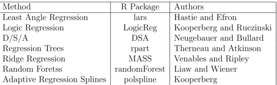
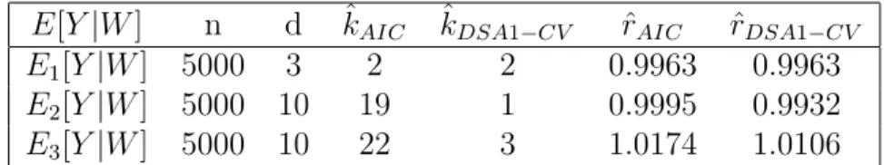
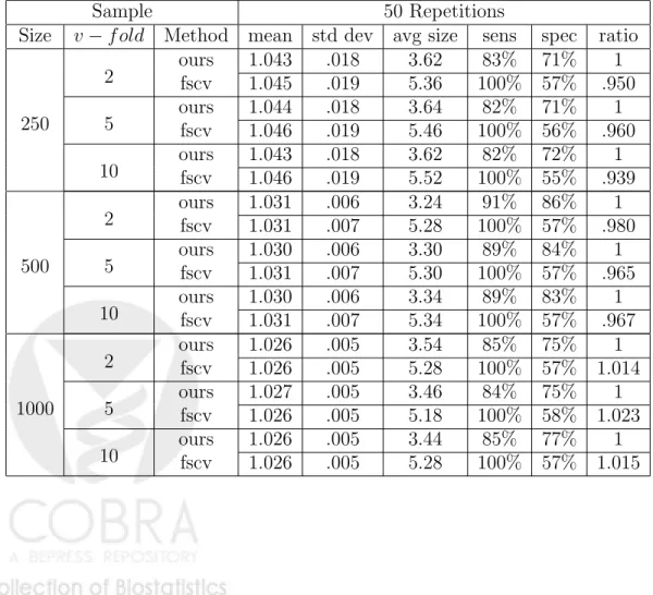
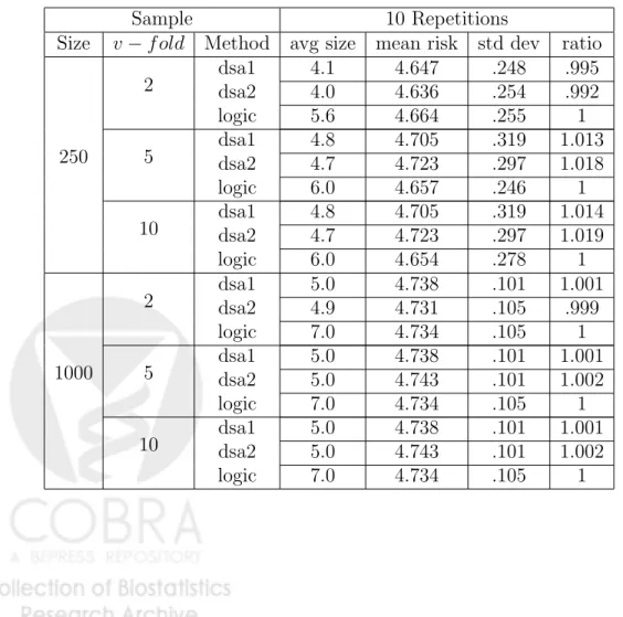
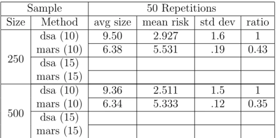
Chapter 3 is titled “Super (Machine) Learning using Cross Validation.” It has two parts. The first part, Super Learner (van der Laan, et al., 2007), proposes an algorithm for constructing a super learner which uses cross-validation to select weights to combine an initial set of candidate estimators, where the true target (typically a function, such as a conditional density, conditional hazard, regression) is defined as a minimizer of the expectation under the observed data distribution P0 of a loss function of O and a can-didate value for the target. For example, the target could represent the whole distribu-tion of the data, a factor of this distribudistribu-tion, an identifiable part of the distribudistribu-tion of the full underlying data, a regression, a median regression, a conditional hazard, a causal dose response curve, and so on. The second part of Chapter 3, Loss-Based Cross-Validated Deletion/Substitution/Addition Algorithms in Estimation (Sinisi and van der Laan, 2004), describes loss-based learning based on cross-validation in the context of regression. This pa-per discusses the Deletion/Substitution/Addition (DSA) algorithm, which is a data-adaptive model selection procedure based on cross-validation and uses polynomial basis functions to search through a parameter space of potential regression functions. This function is available as an R-package. It illustrates concretely how cross-validaiton is used to make a variety of choices when fitting a regression.
Chapter 4 features Collaborative Double Robust Targeted Penalized Maximum Likeli-hood Estimation (van der Laan and Gruber, 2009). It establishes a new collaborative double robustness result for the targeted maximum likelihood estimator, and, in order to exploit this collaborative robustness, refines the standard targeted maximum likelihood estimation pro-cedure by refining the targeted maximum likelihood step. This involves utilizing likelihood-based cross-validation to select among different targeted maximum likelihood steps possibly indexed by different sets of confounders for the treatment/censoring mechanism, thereby yielding maximally effective bias reduction. We show that if the initial estimator converges fast, then the collaborative targeted maximum likelihood estimator can even be super effi-cient. It also presents a strategy to penalize the log-likelihood to make the log-likelihood
Chapter 5, titled “Randomized Controlled Trials,” is concerned with targeted maxi-mum likelihood estimation in randomized controlled trials. Firstly, we present Covariate Adjustment in Randomized Trials with Binary Outcomes: Targeted Maximum Likelihood Estimation (Moore and van der Laan, 2008), which includes simulation studies assessing potential gains in efficiency one can achieve by having predictive baseline covariates. The targeted maximum likelihood estimator for the data structure O = (W, A,∆,∆Y) is pre-sented, where W denotes baseline covariates, A treatment, ∆ indicator of observing the clinical outcome Y. The paper Selecting Optimal Treatments Based on Predictive Factors
(Polley and van der Laan, 2009) shows how one can use super learning and targeted max-imum likelihood to assess effect modification in clinical trials, one factor at the time, or for estimating the treatment effect as a function of a whole set of baseline covariates. In particular, it allows one to estimate the optimal treatment decision in response to baseline characteristics. The paperSimple, Efficient Estimators of Treatment Effects in Randomized Trials Using Generalized Linear Models to Leverage Baseline Variables (Rosenblum and van der Laan, 2009) illustrates that the results for the targeted maximum likelihood estima-tor prove that misspecified generalized linear regression models provide valid estimates of marginal causal effects in randomized controlled trials. That is, these misspecified regression estimators represent particular implementations of the targeted maximum likelihood esti-mator in randomized controlled trials, and are thereby guaranteed to be consistent for the target.
Chapter 6 features Estimating the Effect of Vigorous Physical Activity on Mortality in the Elderly Based on Realistic Individualized Treatment and Intention-to-Treat Rules (Be-mbom and van der Laan, 2007), which presents a practical illustration of the importance of realistic individualized treatment rules in causal inference. It applies targeted maximum likelihood estimation to estimate these causal effects defined by realistic treatment rules in populations where certain levels of treatment are unlikely to be observed in some individuals. Since this is the first application of targeted maximum likelihood estimation to estimate the effect of individualized treatment rules we included this paper in this particular collection of readings, although, we have earlier work (van der Laan and Petersen, 2006, among others) on realistic rules for multiple time-point treatment interventions, but these previous papers apply the IPCW-estimator.
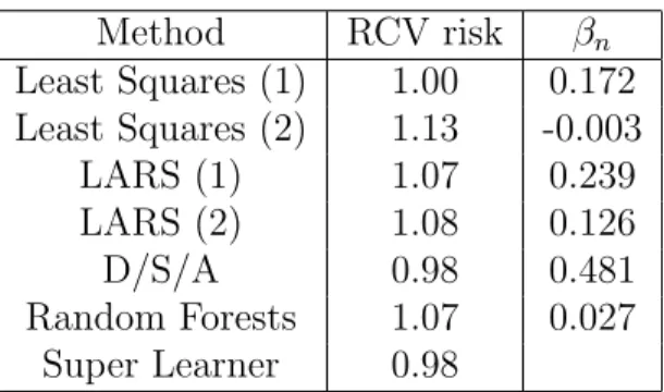
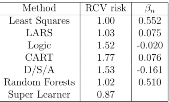
Chapter 7, “Biomarker Discovery,” concerns the application of targeted maximum like-lihood estimation in biomarker discovery. The paper Targeted Methods for Biomarker Dis-covery, the Search for a Standard (Tuglus, van der Laan, 2008) proposes targeted maximum likelihood estimators of variable importance (tVIM) as a standardized method for biomarker discovery. In this paper we focus on variable importance analysis of possibly continuous variables, exploiting the semiparametric regression model to define variable importance. Simulations and data analyses are used to illustrate the benefits achieved in biomarker dis-covery relative to current approaches for variable importance analyses (univariate regression, random forest, lars). The paper Biomarker Discovery using Targeted Maximum Likelihood Estimation: Application to the Treatment of Antiretroviral Resistant HIV Infection (Bem-bom, et al., 2008) discusses and implements targeted maximum likelihood estimation for variable importance for a set of candidate binary biomarkers such as mutations or single
nucleotide polymorphisms. The paper Data-adaptive Selection Of The Adjustment Set In Variable Importance Estimation (Bembom, et al., 2008) introduces an algorithm intended to make variable importance estimation more robust with respect to violations of the ex-perimental treatment assignment assumption. This algorithm is applied to a dataset in an effort to identify mutations in the protease enzyme of HIV that have an effect on virologic response to the commonly used antiretroviral drug lopinavir.
Chapter 8, “Case-Control Studies,” presents targeted maximum likelihood estimation, and, in particular, targeted likelihood based causal inference for case-control studies. The pa-perEstimation Based on Case-Control Designs with Known Prevalance Probability (van der Laan, 2008) provides a comprehensive introduction to case-control weighted targeted maxi-mum likelihood estimation theory for case-control study designs. Simple Optimal Weighting of Cases and Controls in Case-Control Studies (Rose and van der Laan, 2008) implements case-control weighted targeted maximum likelihood estimation for independent case-control study designs, and compares this methodology to existing methods. The paperWhy Match? Investigating Matched Case-Control Study Designs with Causal Effect Estimation (Rose and van der Laan, 2009) discusses the use of matching in case-control study designs. In partic-ular, it compares the efficiency of matched case-control study designs to independent study designs in varied situations using case-control weighted targeted maximum likelihood esti-mation. Lastly, Causal Inference for Nested Case-Control Studies using Targeted Maximum Likelihood Estimation (Rose and van der Laan, 2009) discusses the use of targeted maximum likelihood estimation in nested case-control study designs. It also compares the efficiency of nested case-control designs to analysis of the full cohort data.
Chapter 9 is titled “Time-to-Event Outcomes and Censored Data.” The first paper, A Note on Targeted Maximum Likelihood and Right Censored Data (van der Laan and Rubin, 2007), fully develops the targeted maximum likelihood estimator of causal effects in ran-domized controlled trials with a time-to-event outcome that is subject to right-censoring. The second paper, Application of Time-to-Event Methods in the Assessment of Safety in Clinical Trials (Moore, van der Laan, 2009), provides the theoretical ingredients to derive the targeted maximum likelihood estimator for this data structure.
The Appendix contains a gentle introduction to and R-code for the targeted maxi-mum likelihood estimator of the causal effect of a binary treatment for the data structure (W, A,∆,∆Y) allowing for confounding of treatment and missingness of the clinical out-comeY. For the more theoretical oriented reader, the Appendix also includes a collection of worked out examples of targeted maximum likelihood estimation for different data structures and parameters. This shows how the targeted maximum likelihood step is derived, given the data structure and the model. It presents the natural extension of targeted maximum likeli-hood estimation to targeted minimum loss based learning. In addition, it presents targeted Bayesian learning based on targeted maximum likelihood, presenting a mapping from a prior distribution on the target parameter into a targeted (bias reduced) posterior distribution of the target parameter.
For the interested reader, we note that targeted maximum likelihood has been generalized to group sequential adaptive designs in which the censoring and treatment mechanism of a new subject/unit can be adapted in response to the observed data on the previously recruited units: The Construction and Analysis of Adaptive Group Sequential Designs (van der Laan, 2008). The latter paper contains many additional examples of targeted maximum
sequential design, while preserving frequentist statistical inference based on the martingale central limit theorem.
Finally, we remark that Target Analytics, Inc. (www.targetanalytics.com) is a company founded on the premise of implementing statistical software based on targeted maximum likelihood estimation. A version of TargetDiscovery, a variable importance software product based on targeted maximum likelihood estimation of variable importance across a user sup-plied set of target variables, can be tested directly on the website. The IP for the targeted maximum likelihood estimation methodology is owned by University of California, Berkeley.
Targeted Maximum Likelihood
Estimation
The following article appears as it was published in the International Journal of Biostatistics in 2006, http://www.bepress.com/ijb/vol2/iss1/11/.
It was originally published on the University of California, Berkeley Division of Biostatistics Working Paper Series website in 2006, http://www.bepress.com/ucbbiostat/paper213/.
Targeted Maximum Likelihood Learning
Mark J. van der Laan and Daniel B. Rubin
Suppose one observes a sample of independent and identically distributed observations from a particular data generating distribution. Suppose that one has available an estimate of the density of the data generating distribu-tion such as a maximum likelihood estimator according to a given or data adaptively selected model. Suppose that one is concerned with estimation of a particular pathwise differentiable Euclidean parameter. A substitution estimator evaluating the parameter of the density estimator is typically too biased and might not even converge at the parametric rate: that is, the den-sity estimator was targeted to be a good estimator of the denden-sity and might therefore result in a poor estimator of a particular smooth functional of the
density. In this article we propose a one step (and, by iteration, k-th step)
targeted maximum likelihood density estimator which involves 1) creating a hardest parametric submodel with parameter epsilon through the given den-sity estimator with score equal to the efficient influence curve of the pathwise differentiable parameter at the density estimator, 2) estimating epsilon with the maximum likelihood estimator, and 3) defining a new density estimator as the corresponding update of the original density estimator. We show that iteration of this algorithm results in a targeted maximum likelihood density estimator which solves the efficient influence curve estimating equation and thereby yields a locally efficient estimator of the parameter of interest, un-der regularity conditions. In particular, we show that, if the parameter is linear and the model is convex, then the targeted maximum likelihood esti-mator is often achieved in the first step, and it results in a locally efficient estimator at an arbitrary (e.g., heavily misspecified) starting density. This tool provides us with a new class of targeted likelihood based estimators of pathwise differentiable parameters. We also show that the targeted maximum likelihood estimators are now in full agreement with the locally efficient es-timating function methodology as presented in Robins and Rotnitzky (1992) and van der Laan and Robins (2003), creating, in particular, algebraic equiva-lence between the double robust locally efficient estimators using the targeted maximum likelihood estimators as an estimate of its nuisance parameters, and
targeted maximum likelihood estimators. In addition, it is argued that the targeted MLE has various advantages relative to the current estimating func-tion based approach. We proceed by providing data driven methodologies to select the initial density estimator for the targeted MLE, thereby providing data adaptive targeted maximum likelihood estimation methodology. Finally, in our accompanying technical report we show that targeted maximum likeli-hood estimation can be generalized to estimate any kind of parameter, such as infinite dimensional non-pathwise differentiable parameters, by restricting the likelihood and cross-validated log-likelihood to targeted candidate density estimators only. We illustrate the method with various worked out examples.
1 Introduction
Let O1, . . . , On be n independent and identically distributed (i.i.d.)
observa-tions of an experimental unit O with probability distribution P0 ∈ M, where
M is the statistical model. For the sake of presentation, we will assume that
Mis dominated by a common measureµso that we can identify each possible
probability measure P ∈ M by its density p = dP/dµ. In the discussion we
point out that our methods are not restricted to models dominated by a single
measure. LetPn be the empirical probability distribution ofO1, . . . , On which
puts mass 1/n on each of the n observations. Let p0 = dPdµ0 be the density of
p0 with respect to a dominating measure µ, and let pn be a density estimator
of p0. For example, pn ≡ Φ(Pn) could be the maximum likelihood estimator
defined by the following mapping Φ
pn = Φ(Pn)≡arg maxP∈M n X i=1 logdP dµ(Oi).
Alternatively, if the model M is too large in the sense that the maximum
likelihood estimator is too variable or even inconsistent, then one typically
proposes a sieve Ms ⊂ M, indexed by indices s, approximating M, and
computes candidate maximum likelihood estimators
pns = Φs(Pn) ≡arg max P∈Ms n X i=1log dP dµ(Oi).
In such a setting it remains to data adaptively selects. For example, one could
use likelihood based cross-validation to select s:
sn = arg maxs EBn
X
i:Bn(i)=1
log Φs(Pn,B0 n)(Oi),
where Bn ∈ {0,1}n is a random vector of binary variables defining a random
split in a training sample{i :Bn(i) = 0}and validation sample{i :Bn(i) = 1},
andP0
n,Bn, Pn,B1 n denote the empirical probability distributions of the training
and validation sample, respectively. Now, one would define the estimator of
p0 as the cross-validated maximum likelihood estimator given by
pn = Φ(Pn) ≡pnsn = Φsn(Pn).
It is common practice to evaluate one or many Euclidean valued smooth
functionals Ψ(pn) of the density estimator pn and view them as estimators of
this method is known to result in efficient estimators of Ψ(p0) in
paramet-ric models (i.e., M in the above definition of pn is a parametric model), in
general, such substitution estimators are not correctly trading off bias and
variance with respect to the parameter of interest ψ0 = Ψ(p0). For example,
a univariate (standard) kernel density estimator optimizing the mean squared
error with respect to p0, assuming a continuous second derivative, can have
bias of the ordern−2/5 based on an optimal bandwidth of the ordern−1/5. The
corresponding substitution estimator of the cumulative distribution function
at a point can have bias which converges to zero at the same rate n−2/5, but
a variance of O(1/n), so that the substitution estimator has a variance (1/n)
which is smaller than the square bias (n−4/5) by an order of magnitude. In
particular, the smoothed empirical cumulative distribution functions would
not even converge at root-n rate due to the fact that √n times the bias n−2/5
does not converge to zero: that is, in this kernel density estimator example √
nn−2.5 → ∞, so that the relative efficiency of the empirical cumulative
dis-tribution function and this smooth cumulative disdis-tribution function converges
to zero. This shows that substitution estimators based on optimal (for the
purpose of the density itself) density estimators of the cumulative distribution function are typically theoretically inferior to other more targeted estimators of the parameter of interest. In general, substitution estimators based on den-sity estimators might simply not be very good estimators, and, in particular, likelihood based substitution estimators will often fail to be asymptotically ef-ficient due to the bias caused by the curse of dimensionality: the kernel density example already shows the failure of likelihood based learning of smooth pa-rameters of a density of a univariate random variable, and it gets much worse for densities of multivariate random variables. This issue has been stressed repeatly by Robins and co-authors (see e.g., Robins and Rotnitzky (1992) and van der Laan and Robins (2003)). This article proposes a method which, given a particular pathwise differentiable parameter of interest, allows one to map a
density estimator (such aspn orpns for eachs) into a targeted maximum
likeli-hood density estimator so that the corresponding substitution estimator ofψ0
is locally efficient, under reasonable conditions: that is, if the starting density estimator is consistent, it will typically be efficient, and otherwise in certain classes of problems it might still be consistent and asymptotically linear.
Specifically, in this article we propose a one step maximum likelihood den-sity estimator which involves 1) creating a parametric model with Euclidean
parameter (e.g., the same dimension das the parameter ψ0) through a given
density estimator p0
n (e.g., s-specific MLE pns) at = 0 whose scores include
the components of the efficient influence curve of the pathwise differentiable
parameter at the density estimator p0
likelihood estimator of this parametric model, and 3) defining a new density
estimatorp1
n as the corresponding fluctuation of the original density estimator
p0
n. In addition, iterating this process results in a sequence of pkn with
in-creasing log-likelihood converging to a solution of the efficient influence curve estimating equation, and thereby typically results in a locally efficient
substi-tution estimator of ψ0. We refer to this solution as the targeted maximum
likelihood estimator based on the initial p0
n. We provide various examples in
which this targeted maximum likelihood estimator is achieved at the first step of the algorithm.
In particular, one can map each model based MLE pns into a targeted MLE
p∗
ns (targeted towards ψ0). We suggest that it is appropriate to select among
this collection of targeted MLEsp∗
ns with likelihood based cross-validation, as
explained heuristically in our accompanying technical report: targeted MLE’s are comparable w.r.t. to being fully trained w.r.t. estimation of the parameter of interest, which makes the log-likelihood an appropriate criteria to select
among them. That is, letp∗
ns = ˆΦ∗s(Pn) be thes-specific targeted MLE applied
to the initial density estimator pns. Let
sn = arg maxs EBn
X
i:Bn(i)=1
log ˆΦ∗
s(Pn,B0 n)(Oi),
where Bn ∈ {0,1}n is a random vector of binary variables defining a random
split in a training sample{i :Bn(i) = 0}and validation sample{i :Bn(i) = 1},
andP0
n,Bn, Pn,B1 n denote the empirical probability distributions of the training
and validation sample, respectively, as above. Now, likelihood cross-validated targeted MLE is defined as:
p∗
n = ˆΦ(Pn) ≡p∗nsn = ˆΦ
∗
sn(Pn).
We also note that the candidate models indexed byscan be chosen to represent
a sieve in a possibly misspecified (big) model M, as long as this model M
is still such that the Kullback-Leibler projection of the true density p0 on
this model identifies the parameter of interest Ψ(p0) correctly: for example,
if the parameter of interest is a parameter of a regression of an outcome Y
on covariates W, then one might select as big model the normal densities
with unspecified conditional mean, given W, and certain possibly misspecified
conditional variance, even though the true density p0 is not a member of this
model.
1.1 Organization of article.
In Section 2, given an initial density estimator p0
n (e.g., pns) ofp0, we formally
define the k-th order targeted maximum likelihood density estimator pk
corresponding targeted maximum likelihood estimator Ψ(pk
n) of ψ0. We
illus-trate the targeted MLE of the cumulative distribution function at a point in a nonparametric model. In this case, it appears that the first step targeted MLE
of ψ0 algebraically equals the empirical cumulative distribution function, for
any given initial density estimator p0
n. Thus, while the original substitution
estimator of the cumulative distribution function would not converge at the
parametric rate 1/√n due to it being too biased, the first order targeted bias
corrected density estimator estimates the cumulative distribution function ef-ficiently. In Section 3 we establish that the targeted MLE solves the efficient influence curve estimating equation, which provides the basis of its asymptotic
efficiency for ψ0. In Section 4 we present general templates for establishing
consistency, asymptotic linearity and efficiency of the targeted MLE of ψ0,
which provides a particular powerful theorem for convex models and linear pathwise differentiable parameters stating that the targeted MLE will be con-sistent and asymptotically linear for an arbitrary starting density, and it will be efficient if the starting (or its targeted MLE version) density consistently estimates the efficient influence curve. We illustrate the latter result with two examples. In Section 5 we discuss the relation, and in particular, the algebraic equivalence, between targeted maximum likelihood estimation and estimating function based estimation if one estimates the nuisance parameters in the es-timating functions with the targeted MLE. We point out that targeted MLE is more widely applicable by not relying on being able to map the efficient influence curve in a corresponding estimating function, and it deals naturally with the issue of multiple solutions of estimating equations. In Subsection 5.1 we focus on censored data models to make the comparison with the estimat-ing function methodology in van der Laan and Robins (2003). In particular, we present the targeted MLE approach which results in algebraic equivalence between the Inverse Probability of Censoring Weighted estimator, the dou-ble robust IPCW estimator, and the targeted MLE of a parameter of the full
data distribution based on observing n i.i.d. observations of a censored data
structure under coarsening at random (CAR). These results show that the targeted MLE does not only provide a boost for likelihood based estimation, but it also provides an improvement relative to the current implementation of locally efficient estimation based on estimating function methodology. In Sec-tion 6 we present important examples illustrating the power and computaSec-tional simplicity of this new targeted maximum likelihood estimator: estimation of a marginal causal effect, and the parametric component in a semiparamet-ric regression model, and we present a simulation to illustrate the targeted MLE. In Section 7 we present a loss based approach of targeted MLE learning based on the unified loss function based approach in van der Laan and Dudoit
(2003). We end this article with a discussion in Section 8. In our accompany-ing technical report we show generalizations of the targeted MLE of pathwise differentiable parameters to targeted MLE of general parameters.
1.2 Some relevant literature overview.
There exist various methods for construction of an efficient estimator of a pa-rameter based on parametric models. In particular, Fisher’s method of maxi-mum likelihood estimation can be applied, or closely related M-estimate (i.e., estimators defined as solutions of estimating equations) methods which work under minimal conditions. Maximum likelihood estimation in semiparametric models has been an extensive research area of interest. Here we suffice with a referral to van der Vaart and Wellner (1996b) for a partial overview of the theory for the analysis of maximum likelihood. There are plenty of examples in which the straightforward semiparametric MLE even fails to be consistent, but often an appropriate regularization can be applied to repair the consistency of the semiparametric MLE: e.g., see van der Laan (1995) for such examples based on censored data. However, as argued above in the kernel density es-timator example, maximum likelihood based smoothing/model selection will often provide the wrong trade-off of bias and variance for specific smooth pa-rameters. The literature (notably Robins and co-authors) has recognized this problem with likelihood based estimation. For example, smoothing survival functions or smoothing the nonparametric components in a semiparametric re-gression model requires so called “under-smoothing” in order to obtain root-n consistency for the parameter of interest: see e.g., Cosslett (2004).
For an overview of the literature on efficient estimation of pathwise differ-entiable parameters in semiparametric models we refer to Bickel et al. (1993b). In particular, the latter presents the general one step estimator based on an estimate of the efficient influence curve: see e.g. Klaassen (1987). For an overview of the literature on locally efficient estimating function based esti-mation of pathwise differentiable parameters based on censored longitudinal data (starting with the ground breaking paper Robins and Rotnitzky (1992)), we refer to van der Laan and Robins (2003).
A unified loss function approach based methodology for estimation and estimator selection, and concrete illustration of this method in various exam-ples is presented in van der Laan and Dudoit (2003). This methodology is general by allowing the loss function to be an unknown function of the ex-perimental unit and the parameter values. van der Laan and Rubin (2005) and van der Laan and Rubin (2006) present an alternative unified estimating function methodology for both estimation and estimator selection. The latter
two methodologies provide two general strategies for data adaptive estimation of any parameter in any model.
We note that these (unified) loss function and (unified) estimating func-tion based approaches give up on using the log-likelihood as loss funcfunc-tion for the purpose of estimator selection and estimation when the parameter of in-terest is not the actual density of the data, but a particular parameter of it: these methods replace the log-likelihood loss function by a loss function or an estimating function targeted at the parameter of interest. From that point of view, the current article shows that it is not necessary to replace the log-likelihood loss function by a targeted loss function, but that one can also target the directions in which one maximizes the log-likelihood.
2 Targeted maximum likelihood estimators.
Let Ψ :M →IRdbe a pathwise differentiable parameter at any densityp∈ M,
where M denotes the statistical model consisting of the possible densities
p= dP/dµof O with respect to some dominating measure µ. That is, given a
sufficiently rich class of one-dimensional regular parametric submodels{pδ : δ}
with parameter δ of M through the density p at δ = 0, we have for each of
these submodels pδ with score s at δ = 0 andpδ=0 = p
d
dδ Ψ(pδ)|δ=0 = EpS(p)(O)s(O)
for some S(p) ∈(L2
0(p))d, where L20(p) denotes the Hilbert space of functions
of O with mean 0 and finite variance under P, endowed with inner product
hh1, h2iP = Eph1(O)h2(O). This random variable S(p) ∈ (L20(p))d is called a
gradient of the pathwise derivative atp. LetT(p)⊂L2
0(p) be the tangent space
at p which is defined as the closure of the linear span of the scores s of this
class of submodels throughp. If the model is not locally saturated in the sense
thatT(p) =L2
0(p), then there can be many gradients. LetTnuis⊥ (p)⊂L20(p) be
the orthogonal complement of the so called nuisance tangent space, where the
latter is defined as the closure of the linear span of all scores of pδ for which
the pathwise derivative equals 0 (see van der Laan and Robins (2003), Chapter 1). As in van der Laan and Robins (2003), we denote the set of gradients at
p with T⊥∗
nuis(p) ⊂ (Tnuis⊥ (p))d. Let S∗(p) be the so called canonical gradient
which is the unique gradient whose d components S∗(p)
j, j = 1, . . . , d, are
elements of the tangent space T(P). A submodel {p : } with score S∗(p) at
= 0 is often referred to as a hardest submodel (Bickel et al. (1993a)), as we
Let (O, p) → D(p)(O) be a point-wise well defined class of functions on
the Cartesian product of the support of O and the model M, which satisfies
D(p) =S∗(p) P
0-a.e. for all p∈ M.
As an example, consider letting O be a Euclidean valuedd-variate random
variable with density p0. Let M be the class of all continuous densities with
respect to Lebesgue measureµ, and let Ψ(p) =Rt
0p(o)dµ(o) be the cumulative
distribution function at a point t ∈ IR corresponding with density p. In this
case Ψ : M → IR is pathwise differentiable parameter at p with efficient
influence curveS(p)(O) =I(O ≤t)−Ψ(p), and, because the model is locally
saturated, it is also the only influence curve/gradient. So D(p) =I(O ≤t)−
Ψ(p). Similarly, given a set of user supplied points{t1, . . . , td}, we could define
thed-dimensional Euclidean parameter Ψ(p) = (Ψ(p)(tj) ≡R0tjp(o)dµ(o) :j=
1, . . . , d) representing the cumulative distribution function atdpoints. In this
case, D(p) = (I(O ≤tj)−Ψ(p)(tj) :j = 1, . . . , d) has d components.
A general methodology for construction of functions Dh(p) indexed by an
h ∈ H so that {Dh(p) : h ∈ H} ⊂ Tnuis⊥ (p) (or equality) is presented in
van der Laan and Robins (2003). In van der Laan and Robins (2003) the
class of functions {Dh(p) : h ∈ H} is referred to as a representation of the
orthogonal complement of the nuisance tangent space, which is then used to map into a class of corresponding estimating functions for the pathwise
differentiable parameter p → Ψ(p) of the form p → Dh(Ψ(p),Υ(p)) with Υ
representing a nuisance parameter. In van der Laan and Robins (2003), for a
variety of general classes of models and censored data structures O, explicit
representations of the orthogonal complement of the nuisance tangent space,
T⊥
nuis(p), corresponding gradients, Tnuis⊥∗ (p), and canonical gradientS∗(p), have
been provided.
Let p0
n = Φ(Pn) ∈ M be a density estimator of p0 = dP0/dµ. Define now
a parametric submodel {p0
n() : ∈ IRk} ⊂ M through p0n at = 0 whose
linear span of scores of at = 0 includes all d components of D(pn). One
possibility is to choose ∈ IRd of the same dimension as D(p) and arrange
that the score of j at = 0 equals Dj(p), j = 1, . . . , d. For example, if the
model Mis convex then the following model typically applies
p0
n() ≡(1 +>D(p0n))p0n, (1)
where ∈ IRd denotes the parameter ranging over all values for which p0
n()
is a proper density. Note that indeed p0
n(0) = p0n, p0n() is a density (positive
valued and integrates till 1) for small enough, and d
One can also use an exponential family
p0
n()≡C(, p0n) exp(>D(p0n))p0n
for C(, p0
n) be a normalizing constant. In general, one can choose a
parame-terization → p0
n() ∈ M which is smooth in at = 0 and whose score at
= 0 equalsD(p0
n). However, we will also consider submodelsp0n() with
addi-tional scores in order to arrange that the targeted MLE will be fully targeted
towards estimation of D(p0). Let n =(Pn |pn0) ≡arg{:pmax0 n()∈M} n X i=1 logp0 n()(Oi)
be the maximum likelihood estimator of treating the density estimator p0
n as given and fixed. We will assume that the maximum is attained in the interior
of M so that n solves the estimating equation:
0 =Pn
d dp0n()
p0
n() .
Here we use the common notation P f ≡R f(o)dP(o). For example, ifp0
n() =
(1 +>D(p0
n))p0n, as one might choose in convex models, then we have that n
is the solution of 0 = 1 n n X i=1 D(p0 n)(Oi) 1 +> nD(p0n)(Oi). This defines now an updated density estimator
p1
n ≡p0n(n) =p0n((Pn |p0n)) ∈ M.
Note that this simply defines a method for mapping an initial density estimator
p0
n ∈ M in a new density estimator p1n ∈ M, which we call the first step
targeted maximum likelihood estimator. By iterating this process one obtains
the k-step targeted maximum likelihood estimator pk
n, k= 1, . . .
Definition 1 Given an initial density estimator p0
n = ˆΦ0(Pn) based on the
empirical probability distributionPn, a parametric fluctuation{p0n() :} ⊂ M
satisfying p0
n(0) = p0n, and dd logp0n()=0 = D∗(p0n), where the linear span of
the components of D∗(p0
n) include all d components of a canonical gradient
D(p0
n) of the parameter of interest Ψ :M → IRd at p0n, a maximum likelihood
estimator (Pn |p0n) ≡arg max n X i=1logp 0 n()(Oi)
of , we define the first step targeted maximum likelihood density estimator as
p1
n = ˆΦ1(Pn)≡p0n((Pn | p0n)).
This process can be iterated to define the k-step targeted maximum likelihood density estimator as
pk+1
n = ˆΦk+1(Pn)≡pkn((Pn |pkn)), k = 0,1, . . ..
The corresponding k-step targeted maximum likelihood estimator of ψ0 is
defined as
ˆΨk(Pn) = Ψ(pkn).
The targeted maximum likelihood estimator is defined as
ψn = ˆΦ∗(Pn)≡klim→∞Ψ(pkn),
assuming this limit exists.
2.1 Example: Estimating the CDF.
Consider an initial data generating density p0 = f, let F(t) = Rt
−∞f(o)do
denote the associated CDF at some fixed point t∈IR, and consider the
para-metric model ( f(o) = (1 +[I(o≤t)−F(t)])f(o) :− 1 1−F(t) ≤≤ 1 F(t) ) , (2)
where one can check that the range restraint on serves merely to ensure that
the family is indeed a proper class of densities. Consider estimating from
maximum likelihood based on an i.i.d. sample {Oi}ni=1. The log likelihood is,
l() =Xn i=1 log(1 +[I(Oi ≤t)−F(t)]) + n X i=1 logf(Oi). (3)
Its derivative is,
l0() =Xn
i=1
I(Oi ≤t)−F(t)
1 +[I(Oi≤t)−F(t)]. (4)
Its second derivative is easily seen to be,
l00() =−Xn i=1 ( I(Oi≤t)−F(t) 1 +[I(Oi ≤t)−F(t)] )2 . (5)
Because the log likelihood is concave, we know that the maximum is achieved
if l0() = 0 has a solution. Letting F
n(·) denote the empirical distribution
function, note that we can decompose the terms in l0() into two parts (those
for which I(Oi ≤t) are 0 or 1), and the MLE of can be seen to solve,
0 = l0() = Xn i=1 I(Oi ≤t)−F(t) 1 +[I(Oi≤t)−F(t)] = nFn(t) 1−F(t) 1 +[1−F(t)] +n(1−Fn(t)) −F(t) 1−F(t).
Moving the second term on the right to the other side of the equation, dividing
both sides by n, and multiplying both sides by (1 +[1 −F(t)])(1−F(t)),
the equation reduces to,
Fn(t)(1−F(t))(1−F(t)) = (1−Fn(t))F(t)(1 +(1−F(t))). (6)
This is linear in , and one can check that the solution is
n = Fn(t)(1−FF((tt)(1))−−(1F(−t))Fn(t))F(t)
= Fn(t)−Fn(t)F(t)−F(t) +Fn(t)F(t)
F(t)(1−F(t))
= Fn(t)−F(t)
F(t)(1−F(t)). (7)
Because 0≤Fn(t) ≤1, one can check that indeed
− 1 1−F(t) = − F(t) F(t)(1−F(t) ≤n ≤ 1−F(t) F(t)(1−F(t)) = 1 F(t), (8)
so the range restraint on for the family (2) always holds for the maximum
likelihood estimator, meaning thatfn(·) is a proper density. Now, the
result-ing CDF at tfor this density is then,
Fn(t) = Z t −∞fn(o)do = Z t −∞(1 +n[I(o≤t)−F(t)])f(o)do = Z t −∞f(o)do+n Z t −∞I(o≤t)f(o)do−1F(t) Z t −∞f(o)do
= F(t) +nF(t)−nF(t)2 = F(t) +1F(t)(1−F(t))
= F(t) + Fn(t)−F(t)
F(t)(1−F(t))F(t)(1−F(t)) from (7)
= F(t) +Fn(t)−F(t) =Fn(t).
Therefore, for any initial density f(·) and any time point t, the targeted
like-lihood maximum likelike-lihood estimator of the CDF reduces to the empirical distribution estimator in a single step. This result immediately generalizes to
Ψ(p) =RAp(o)dµ(o) for any measurable set A.
3 Solving the efficient estimating equation.
We have the following trivial, but useful result. It states that if the MLE’s
(Pn | pkn) at stepkof the targeted MLE algorithm converge to zero fork→ ∞
(as one expects to hold if the log likelihood of the data is uniformly bounded
in the model M), then the algorithm converges to a solution of the efficient
influence curve equation PnD(p) = 0 in the sense thatPnD(pkn) →0.
Result 1 Let Pn be given. Assume that lim →0lim supk→∞ |Pn d dpkn() pk n() −Pn pk0 n(0) pk n(0) |→0, (9)
that for each k there exist a constant matrix Ak so that Akp k0 n pk n = D(p k n) with
lim supk→∞k Ak k< ∞, where kA k denotes a matrix norm.
If (Pn |pkn) solves Pn d dpkn()
pkn() = 0 for all k, and (Pn | pkn)→0 for k→ ∞,
then we have
PnD(pkn)→0 for k → ∞.
The condition (9) holds if the score of the one-dimensional submodel p()
at converges to the score at = 0 for → 0 uniformly in a set containing
the k-step targeted MLE’s pk
n, k = 1,2, . . ., and that for each p ∈ M, the
linear span of the components pp0(0)(0) includes the components of D(p). Since
the likelihood increases at each step one might indeed expect that typically the
targeted MLE algorithm will converge and thereby that (Pn | pkn)→0. That
is, Result 1 essentially states that, if the targeted MLE algorithm converges, then the algorithm will converge to a solution of the efficient influence curve
arbitrary small deviation from 0.
Proof. Let k =(Pn |pnk), k= 0, . . .. If k →0 for k→ ∞, then
Pn d dkp k n(k) pk n(k) −Pn pk0 n(0) pk n(0) →0
fork → ∞. Let Ak be such thatAkp
k0 n(0) pk
n(0) = D(p k
n). By assumption, the matrix
has a norm bounded uniformly in k. Thus, we also have
PnAk d dkp k n(k) pk n(k) −PnD(p k n)→0
for k → ∞. However, Pnddkpkn(k)/pkn(k) = 0 (and thus Ak applied to this
equals 0 as well), which shows that PnD(pkn)→0. 2
4 Efficiency of targeted likelihood estimation.
In this section we provide templates for proving consistency, asymptotic linear-ity and efficiency of the targeted maximum likelihood estimator of a path-wise differentiable parameter. Since convexity of the model and linearity of the parameter allows a particular strong result, we separate this situation from the general case.
4.1 Linear parameters in convex models.
Let p∞
n denote the limit of our algorithm if it exists as a density with respect
to µ in M, and otherwise it represents a pk
n ∈ M for a large enough k. If
the condition of the above Result 1 holds, then p∞
n ∈ M, and for all practical
purposes, we have PnD(p∞n ) = 0. If this is true, then this result can be used
to establish efficiency of the substitution estimator Ψ(p∞
n ) as an estimator
of ψ0 under the assumption that the parameter Ψ : M → IRd is linear and
M is convex, under weak regularity conditions. Specifically, by the identity
for convex models and linear parameters in van der Laan (1998) we have
Ψ(p)−Ψ(p0) = −P0D(p) for any p, p0 ∈ M for which p0/p < ∞. Thus, if
p∞
n ∈ M and it is bounded away from 0 on the support of p0, then combining
PnD(p∞n ) = 0 with the latter identity gives us
Ψ(p∞
n )−Ψ(p0) = (Pn−P0)D(p∞n ). (10)
Even if p∞
n does not satisfy p0/p∞n < ∞, then the identity Ψ(p∞n )−Ψ(p0) =
(see van der Laan (1998)), so that (10) can even be established for density estimators not satisfying this support condition.
Applying empirical process theory (van der Vaart and Wellner (1996a)) now
proves that Ψ(p∞
n ) is root-nconsistent ifD(p∞n ) falls in aP0Donsker class with
probability tending to 1. If one can now also establish thatP0(D(pn∞)−D(p1))2
converges to zero in probability for a certain p1 ∈ M, then it follows that
Ψ(p∞
n ) is asymptotically linear with influence curveD0(p1)≡D(p1)−P0D(p1):
Ψ(p∞
n )−Ψ(p0) = (Pn−P0)D0(p1) +oP(1/√n),
where we note that p1 can be an arbitrary limit (i.e., p1 6= p0 is allowed). In
particular, if the limitp1is such thatD(p1) =D(p0), then Ψ(p∞n ) is
asymptot-ically linear with influence curveD(p0). Thus, ifD(p0) is the efficient influence
curve, then Ψ(p∞
n ) is asymptotically efficient.
Theorem 1 Suppose the conclusion of Result 1 holds, and K = K(n) is chosen large enough so that the targeted MLE pn = pKn satisfies PnD(pn) =
R(n, K(n)) =oP(1/√n) (where limK→∞R(n, K) = 0). Assume that pn ∈ M,
p0/pn < ∞ uniformly over a support of p0, M is convex, and Ψ :M →IRd is
linear. Then
Ψ(pn)−Ψ(p0) = (Pn−P0)D(pn) +R(n, K(n)).
If D(pn) falls in a P0 Donsker class with probability tending to 1, then
Ψ(pn)−ψ0 =OP(1/√n).
If it is also shown that P0(D(pn)−D(p1))2 →0 in probability for n→ ∞ for
some p1 ∈ M, then it follows thatΨ(pn)is asymptotically linear with influence
curve D(p1)−P0D(p1):
Ψ(pn)−Ψ(p0) = (Pn−P0)D(p1) +oP(1/√n).
In particular, if D(p1) = D(p0), and D(p0) is the efficient influence curve of
Ψ at p0, then Ψ(pn) is asymptotically efficient.
This shows that the targeted MLE of a linear parameter in a convex model is typically consistent and asymptotically linear for arbitrary starting density
p0
n, and if the targeted MLE p∞n is consistent in the sense that P0(D(p∞n )−
D(p0))2 → 0 with probability tending to 1 for n converging to infinity (e.g.,
the initial starting densityp0
nwould already yield a consistent estimator D(pn0)
two examples illustrating this theorem. The first example represents a case
in which the targeted MLE is efficient for arbitrary starting density p0
n. The
second example represents the case that the targeted MLE is consistent and
asymptotically linear for arbitrary starting density p0
n, and is efficient if the
starting density consistently estimates D(p0).
Example 1 ((Efficiency of a smooth cumulative distribution func-tion) In this example we have D(p)(O) = I(O ≤ t) −Rt
0p(o)dµ(o). A
tar-geted MLE pn solving PnD(pn) = 0 satisfies that Ψ(pn) = PnI(· ≤ t) equals
the empirical cumulative distribution function at t and is therefore
asymp-totically efficient, for arbitrary starting density p0. Thus in this example the
initial density does not need to be consistent in order to make the targeted
MLE asymptotically efficient. Suppose that p0
nh is indexed by a bandwidth
or model choice h, and let p∗
nh be the targeted MLE density estimator using
as starting density p0
nh. Each of the targeted MLE’s p∗nh results in the same
estimator of the cumulative distribution function Ψ(p0) at time t. If one uses
likelihood cross-validation to selecth, then one selects among all of these
tar-geted MLE’s the one which is supposedly closest to the true density p0 with
respect to Kullback-Leibler divergence, which now provides a valid and rea-sonable criteria since all the candidates density estimators already map into
efficient (and algebraically equivalent) estimators of ψ0.
Example 2 ((Local efficiency of targeted MLE based on censored data) We consider a particular example of a censored data structure to il-lustrate that Theorem 1 yields local efficiency of the targeted MLE based on
CAR censored data structures based on any starting density p0
n, under very
weak conditions.
Suppose that the full data structure X = (W, Y(a) : a ∈ {0,1}) on the
experimental unit consists of a set of baseline covariates W, and treatment
specific outcomes Y(a), indexed by treatment valuesa∈ {0,1}. Suppose that
the observed data structure O = (W, A, Y = Y(A)) ∼ p0, and it is assumed
that the conditional probability distribution g0(· | X) of A, given X, satisfies
g0(A | X) = g0(A | W): that is, A is independent of X, given W. Suppose
that this conditional probability distribution of g0(A | W) of A, given W, is
known, and satisfies 0 < g0(1 | W) < 1, as it would be in a randomized trial
aiming to establish the causal effect of A on Y. Let M be the class of all
densities of O with respect to an appropriate dominating measure. We have
M= {p(O) =QXA(W, Y)g0(A|X) :QX0, QX1},
where the full data sub-distributions QXa(w, y) =PW,Y(a)(w, y) are joint